import numpy as np
import pandas as pd
import scipy as scp
import matplotlib.pyplot as plt
import math
import matplotlib.cm as cmx
from mssm.models import *
from mssm.src.python.compare import compare_CDL
from mssmViz.plot import *
from mssmViz.sim import *
from mssmViz.extract import *
import matplotlib.style as mplstyle
mplstyle.use('fast')
np.set_printoptions(suppress=True)

nc = 10
colors = [cmx.tab20(x) for x in np.linspace(0.0,min(0.1*nc,1.0),nc)]
single_size = 8/2.54
mssm Tutorial
With mssm we can estimate a broad variety of smooth models as they are also supported in mgcv (Wood, 2017). Terms that are available in both mgcv and mssm include regular univariate smooth terms, binary smooth terms, Tensor smooth interactions, by-factor smooth terms (ordered and not ordered), and random non-linear smooth terms. Like mgcv, mssm also supports random effects (random intercepts, random slopes, and as mentioned random smooths). By default a B-spline basis is used by mssm for all smooth terms and penalties are either difference (Eilers & Marx, 2010) or identity penalties (Kernel penalties, Marra & Wood (2012) are also supported).
Like mgcv, mssm supports estimation of conventional Generalized additive (mixed) models. Currently, Binomial models (N >= 1), Gamma models, Inverse Gaussian, Poisson, and Gaussian models are supported! mssm uses sparse matrices and is thus particularly well equipped to handle models of multi-level data, including many random effects! mssm also supports estimation of GAMMs of location, scale, and shape parameters (“GAMMLSS”; see Rigby & Stasinopoulos, 2005) and even more general smooth models (“GSMMs”) as defined by Wood, Pya, & Säfken (2016).
mssm automatically figures out the right amount of penalization for all terms and all these models using a combination of the approaches discussed by Wood, Pya, & Säfken (2016), Wood & Fasiolo (2017), Wood, Shaddick, & Augustin, (2017). Alternatively, the L-qEFS update by Krause et al. (submitted) can be used to select the regularization/penalization parameters. This update is particularly attrative when working with general smooth models, since it only requires researchers to code up the log-likelihood and (optionally) ways to compute its gradient in order to estimate and regularize the model. Krause et al. (submitted) provides a detailed description of the different algorithms implemented in the mssm toolbox.
In contrast, this tutorial focuses on practical application of the mssm toolbox. It contains:
a brief discussion of the structure your data should have
an introduction to the
Formulaclass, including a conversion table if you are familiar withmgcvsyntax and just want to get startedan extensive section of examples involving Gaussian additive models so that you can get familiar with the
Formulaclass and the different terms supported bymssmexamples on how to estimate Generalized additive models and even more general models (i.e., GAMMLSS and GSMMs)
a section on advanced topics, focused on model selection, posterior sampling, and working with the
GSMMclass
Along the way, this tutorial introduces the plot functions available in mssmViz, which can be used to visualize model predictions and to asses model validity via residual plots for all models estimated by mssm. This tutorial assumes that you are already familiar with the idea behind GAMMS (and perhaps even GAMMLSS models; Rigby & Stasinopoulos, 2005) and does not aim to provivde a thorough introduction to their theory. Instead, the aim is to quickly show you how to fit, inspect, validate, and select between these models with mssm. If you want to learn more about the theory behind GAMMS (and GAMMLSS models), head to the reference section at the end of the tutorial, which contains pointers to papers and books focused on GAMM & GAMMLSS models.
Data structure
# Import some simulated data
dat = pd.read_csv('https://raw.githubusercontent.com/JoKra1/mssmViz/main/data/GAMM/sim_dat.csv')

# mssm requires that the data-type for variables used as factors is 'O'=object
dat = dat.astype({'series': 'O',
                  'cond':'O',
                  'sub':'O',
                  'series':'O'})
Some remarks about the desired layout of the data to be usable with the GAMM class:
Data has to be provided in a
pandas.DataFrame.The dependent variable can contain NAs, which will be taken care of. No NAs should be present in any of the predictor columns!
The data-type (dtype) for numeric columns should be float or int. Categorical predictors need to have the object datatype (see code above).
No specific row/column sorting is required.
Exception to the last point:
If you want to approximate the computations for random smooth models of multi-level time-series data or want to include an “ar1” model of the residuals (see section on advanced topics), the data should be ordered according to series, then time: the ordered (increasing) time-series corresponding to the first series should make up the first X rows. The ordered time-series corresponding to the next series should make up the next Y rows, and so on. More specifically, what matters is that individual series are making up a time-ordered sub-block of dat. So you could also have a dataframe that starts with a series labeled 0, then a series labeled 115, then a series labeled X. As long as any series in the data is not interrupted by rows corresponding to any other series it will be fine.
# Take a look at the data:
dat.head()
| y | time | series | cond | sub | x | |
|---|---|---|---|---|---|---|
| 0 | 7.005558 | 0 | 0 | a | 0 | 9.817736 |
| 1 | 11.122316 | 20 | 0 | a | 0 | 10.262371 |
| 2 | 4.766720 | 40 | 0 | a | 0 | 10.445887 |
| 3 | 2.952046 | 60 | 0 | a | 0 | 8.481554 |
| 4 | 7.463034 | 80 | 0 | a | 0 | 10.180660 |
# To make sure the last point raised above is met - we can call the following.
# This does not hurt, even if we do not want to rely on approximate computations or don't need an "ar1" model.
dat = dat.sort_values(['series', 'time'], ascending=[True, True])
The Formula class
At the core of each model - independent of whether you want to work with GAMMs, GAMMLSS, or even GSMM - is the Formula. A Formula is used to specify the additive model of a particular parameter of the likelihood/response family of the model. With GAMMs we model a single parameter: the mean of the independent response variables. Thus we need to specify only a single Formula. With GAMMLSS and GSMM, we can model multiple parameters of the response variables/likelihood, and thus we will often have to specify multiple Formulas.
Like most classes and functions implemented in mssm, the Formula class has been extensively documented, including a list of code examples. Thus, to learn more about the Formula class you can rely on the help function as follows:
help(Formula)
Help on class Formula in module mssm.src.python.formula:

class Formula(builtins.object)
 |  Formula(
 |      lhs: lhs,
 |      terms: list[GammTerm],
 |      data: pd.DataFrame,
 |      series_id: str | None = None,
 |      codebook: dict | None = None,
 |      print_warn: bool = True,
 |      keep_cov: bool = False,
 |      find_nested: bool = True,
 |      file_paths: list[str] = [],
 |      file_loading_nc: int = 1,
 |      file_loading_kwargs: dict = {'header': 0, 'index_col': False}
 |  ) -> None
 |
 |  The formula of a regression equation.
 |
 |  **Note:** The class implements multiple ``get_*`` functions to access attributes stored in
 |  instance variables. The get functions always return a copy of the instance variable and the
 |  results are thus safe to manipulate.
 |
 |  Examples::
 |
 |    from mssm.models import *
 |    from mssmViz.sim import *
 |
 |    from mssm.src.python.formula import build_penalties,build_model_matrix
 |
 |    # Get some data and formula
 |    Binomdat = sim3(10000,0.1,family=Binomial(),seed=20)
 |    formula = Formula(lhs("y"),[i(),f(["x0"]),f(["x1"]),f(["x2"]),f(["x3"])],data=Binomdat)
 |
 |    # Now with a tensor smooth
 |    formula = Formula(lhs("y"),[i(),f(["x0","x1"],te=True),f(["x2"]),f(["x3"])],data=Binomdat)
 |
 |    # Now with a tensor smooth anova style
 |    formula = Formula(lhs("y"),[i(),f(["x0"]),f(["x1"]),f(["x0","x1"]),f(["x2"]),f(["x3"])],
 |      data=Binomdat)
 |
 |
 |    ######## Stream data from file and set up custom codebook #########
 |
 |    file_paths = [
 |      f'https://raw.githubusercontent.com/JoKra1/mssmViz/main/data/GAMM/sim_dat_cond_{cond}.csv'         for cond in ["a","b"]
 |      ]
 |
 |    # Set up specific coding for factor 'cond'
 |    codebook = {'cond':{'a': 0, 'b': 1}}
 |
 |    formula = Formula(lhs=lhs("y"), # The dependent variable - here y!
 |                      terms=[i(), # The intercept, a
 |                               l(["cond"]), # For cond='b'
 |                               # to-way interaction between time and cond;
 |                               # one smooth over time per cond level
 |                               f(["time"],by="cond"),
 |                               # to-way interaction between x and cond;
 |                               # one smooth over x per cond level
 |                               f(["x"],by="cond"),
 |                               # three-way interaction
 |                               f(["time","x"],by="cond"),
 |                               # Random non-linear effect of time - one
 |                               # smooth per level of factor sub
 |                               fs(["time"],rf="sub")],
 |                      data=None, # No data frame!
 |                      file_paths=file_paths, # Just a list with paths to files.
 |                      print_warn=False,
 |                      codebook=codebook)
 |
 |    # Alternative:
 |    formula = Formula(lhs=lhs("y"),
 |                            terms=[i(),
 |                                  l(["cond"]),
 |                                  f(["time"],by="cond"),
 |                                  f(["x"],by="cond"),
 |                                  f(["time","x"],by="cond"),
 |                                  fs(["time"],rf="sub")],
 |                            data=None,
 |                            file_paths=file_paths,
 |                            print_warn=False,
 |                            keep_cov=True, # Keep encoded data structure in memory
 |                            codebook=codebook)
 |
 |    # preparing for ar1 model (with resets per time-series) and data type requirements
 |
 |    dat = pd.read_csv(
 |      'https://raw.githubusercontent.com/JoKra1/mssmViz/main/data/GAMM/sim_dat.csv'
 |      )
 |
 |    # mssm requires that the data-type for variables used as factors is 'O'=object
 |    dat = dat.astype({'series': 'O',
 |                      'cond':'O',
 |                      'sub':'O',
 |                      'series':'O'})
 |
 |    formula = Formula(lhs=lhs("y"),
 |                      terms=[i(),
 |                               l(["cond"]),
 |                               f(["time"],by="cond"),
 |                               f(["x"],by="cond"),
 |                               f(["time","x"],by="cond")],
 |                      data=dat,
 |                      print_warn=False,
 |                      series_id='series') # 'series' variable identifies individual time-series
 |
 |  :param lhs: The lhs object defining the dependent variable.
 |  :type variable: lhs
 |  :param terms: A list of the terms which should be added to the model.
 |      See :py:mod:`mssm.src.python.terms` for info on which terms can be added.
 |  :type terms: [GammTerm]
 |  :param data: A pandas dataframe (with header!) of the data which should be used to estimate the
 |      model. The variable specified for ``lhs`` as well as all variables included for a ``term``
 |      in ``terms`` need to be present in the data, otherwise the call to Formula will throw an
 |      error.
 |  :type data: pd.DataFrame or None
 |  :param series_id: A string identifying the individual experimental units. Usually a unique
 |      trial identifier. Only necessary if approximate derivative computations are to be utilized
 |      for random smooth terms or if you need to estimate an 'ar1' model for multiple time-series
 |      data.
 |  :type series_id: str, optional
 |  :param codebook: Codebook - keys should correspond to factor variable names specified in terms.
 |      Values should again be a ``dict``, with keys for each of K levels of the factor and value
 |      corresponding to an integer in {0,K}.
 |  :type codebook: dict or None
 |  :param print_warn: Whether warnings should be printed. Useful when fitting models from terminal.
 |      Defaults to True.
 |  :type print_warn: bool,optional
 |  :param keep_cov: Whether or not the internal encoding structure of all predictor variables
 |      should be created when forming :math:`\mathbf{X}^T\mathbf{X}` iteratively instead of
 |      forming :math:`\mathbf{X}` directly. Can speed up estimation but increases memory
 |      footprint. Defaults to True.
 |  :type keep_cov: bool,optional
 |  :param find_nested: Whether or not to check for nested smooth terms. This only has an effect if
 |      you include at least one smooth term with more than two variables. Additionally, this check
 |      is often not necessary if you correctly use the ``te`` key-word of smooth terms and ensure
 |      that the marginals used to construct ti smooth terms have far fewer basis functions than
 |      the "main effect" univariate smooths. Thus, if you know what you're doing and you're
 |      working with large models, you might want to disable this (i.e., set to False) because this
 |      check can get quite expensive for larger models. Defaults to True.
 |  :type find_nested: bool,optional
 |  :param file_paths: A list of paths to .csv files from which :math:`\mathbf{X}^T\mathbf{X}`
 |      and :math:`\mathbf{X}^T\mathbf{y}` should be created iteratively. Setting this to a
 |      non-empty list will prevent fitting X as a whole. ``data`` should then be set to ``None``.
 |      Defaults to an empty list.
 |  :type file_paths: [str],optional
 |  :param file_loading_nc: How many cores to use to a) accumulate :math:`\mathbf{X}` in parallel
 |      (if ``data`` is not ``None`` and ``file_paths`` is an empty list) or b) to accumulate
 |      :math:`\mathbf{X}^T\mathbf{X}` and :math:`\mathbf{X}^T\mathbf{y}`
 |      (and :math:`\mathbf{\eta}` during estimation) (if ``data`` is ``None`` and ``file_paths``
 |      is a non-empty list). For case b, this should really be set to the maimum number of cores
 |      available. For a this only really speeds up accumulating :math:`\mathbf{X}` if
 |      :math:`\mathbf{X}` has many many columns and/or rows. Defaults to 1.
 |  :type file_loading_nc: int,optional
 |  :param file_loading_kwargs: Any key-word arguments to pass to pandas.read_csv when
 |      :math:`\mathbf{X}^T\mathbf{X}` and :math:`\mathbf{X}^T\mathbf{y}` should be created
 |      iteratively (if ``data`` is ``None`` and ``file_paths`` is a non-empty list).
 |      Defaults to ``{"header":0,"index_col":False}``.
 |  :type file_loading_kwargs: dict,optional
 |  :ivar lhs lhs: The left-hand side object of the regression formula passed to the constructor.
 |      Initialized at construction.
 |  :ivar [GammTerm] terms: The list of terms passed to the constructor. Initialized at
 |      construction.
 |  :ivar pd.DataFrame data: The dataframe passed to the constructor. Initialized at
 |      construction.
 |  :ivar [int] coef_per_term: A list containing the number of coefficients corresponding to each
 |      term included in ``terms``. Initialized at construction.
 |  :ivar [str] coef_names: A list containing a named identifier (e.g., "Intercept") for each
 |      coefficient estimated by the model. Initialized at construction.
 |  :ivar int n_coef: The number of coefficients estimated by the model in total. Initialized at
 |      construction.
 |  :ivar int unpenalized_coef: The number of un-penalized coefficients estimated by the model.
 |      Initialized at construction.
 |  :ivar np.ndarray or None y_flat: An array, containing all values on the dependent variable
 |      (i.e., specified by ``lhs.variable``) in order of the data-frame passed to ``data``. This
 |      variable will be initialized at construction but only if ``file_paths=None``, i.e., in case
 |      :math:`\mathbf{X}^T\mathbf{X}` and :math:`\mathbf{X}^T\mathbf{y}` are **not** created
 |      iteratively.
 |  :ivar np.ndarray or None cov_flat: An array, containing all (encoded, in case of categorical
 |      predictors) values on each predictor (each columns of ``cov_flat`` corresponds to a
 |      different predictor) variable included in any of the ``terms`` in order of the data-frame
 |      passed to ``data``. This variable will be initialized at construction but only if
 |      ``file_paths=None``, i.e., in case :math:`\mathbf{X}^T\mathbf{X}` and
 |      :math:`\mathbf{X}^T\mathbf{y}` are **not** created iteratively.
 |  :ivar np.ndarray or None NOT_NA_flat: An array, containing an indication (as bool) for each
 |      value on the dependent variable (i.e., specified by ``lhs.variable``) whether the
 |      corresponding value is not a number ("NA") or not. In order of the data-frame passed to
 |      ``data``. This variable will be initialized at construction but only if ``file_paths=None``,
 |      i.e., in case :math:`\mathbf{X}^T\mathbf{X}` and :math:`\mathbf{X}^T\mathbf{y}` are
 |      **not** created iteratively.
 |
 |  Methods defined here:
 |
 |  __init__(
 |      self,
 |      lhs: lhs,
 |      terms: list[GammTerm],
 |      data: pd.DataFrame,
 |      series_id: str | None = None,
 |      codebook: dict | None = None,
 |      print_warn: bool = True,
 |      keep_cov: bool = False,
 |      find_nested: bool = True,
 |      file_paths: list[str] = [],
 |      file_loading_nc: int = 1,
 |      file_loading_kwargs: dict = {'header': 0, 'index_col': False}
 |  ) -> None
 |      Initialize self.  See help(type(self)) for accurate signature.
 |
 |  encode_data(self, data: pd.DataFrame, prediction: bool = False) -> tuple[np.ndarray | None, np.ndarray, np.ndarray | None, list[np.ndarray] | None, list[np.ndarray] | None, list[np.ndarray] | None, np.ndarray | None]
 |      Encodes ``data``, which needs to be a ``pd.DataFrame`` and by default
 |      (if ``prediction==False``) builds an index of which rows in ``data`` are NA in the column
 |      of the dependent variable described by ``self.lhs``.
 |
 |      :param data: The data to encode.
 |      :type data: pd.DataFrame
 |      :param prediction: Whether or not a NA index and a column for the dependent variable should
 |          be generated.
 |      :type prediction: bool, optional
 |      :return: A tuple with 7 (optional) entries: the dependent variable described by
 |          ``self.lhs``, the encoded predictor variables as a (N,k) array (number of rows matches
 |          the number of rows of the first entry returned, the number of columns matches the
 |          number of k variables present in the formula), an indication for each row whether
 |          the dependent variable described by ``self.lhs`` is NA, like the first entry but split
 |          into a list of lists by ``self.series_id``, like the second entry but split into a
 |          list of lists by ``self.series_id``, ike the third entry but split into a list of lists
 |          by ``self.series_id``, start and end points for the splits used to split the previous
 |          three elements (identifying the start and end point of every level of
 |          ``self.series_id``).
 |      :rtype: (np.ndarray|None, np.ndarray, np.ndarray|None, list[np.ndarray]|None,
 |          list[np.ndarray]|None, list[np.ndarray]|None, np.ndarray|None)
 |
 |  get_coding_factors(self) -> dict
 |      Get a copy of the factor coding dictionary. Keys are factor variables in the data,
 |      values are dictionaries, where the keys correspond to the encoded levels (int) of the factor
 |      and the values to their levels (str).
 |
 |  get_data(self) -> pd.DataFrame
 |      Get a copy of the ``data`` specified for this formula.
 |
 |  get_depvar(self) -> np.ndarray
 |      Get a copy of the encoded dependent variable (defined via ``self.lhs``).
 |
 |  get_factor_codings(self) -> dict
 |      Get a copy of the factor coding dictionary. Keys are factor variables in the data,
 |      values are dictionaries, where the keys correspond to the levels (str) of the factor and
 |      the values to their encoded levels (int).
 |
 |  get_factor_levels(self) -> dict
 |      Get a copy of the factor levels dictionary. Keys are factor variables in the data,
 |      values are np.arrays holding the unique levels (as str) of the corresponding factor.
 |
 |  get_has_intercept(self) -> bool
 |      Does this formula include an intercept or not.
 |
 |  get_ir_smooth_term_idx(self) -> list[int]
 |      Get a copy of the list of indices that identify impulse response terms in
 |      ``self.terms``.
 |
 |  get_lhs(self) -> lhs
 |      Get a copy of the ``lhs`` specified for this formula.
 |
 |  get_linear_term_idx(self) -> list[int]
 |      Get a copy of the list of indices that identify linear terms in ``self.terms``.
 |
 |  get_n_coef(self) -> int
 |      Get the number of coefficients that are implied by the formula.
 |
 |  get_notNA(self) -> np.ndarray
 |      Get a copy of the encoded 'not a NA' vector for the dependent variable (defined via
 |      ``self.lhs``).
 |
 |  get_random_term_idx(self) -> list[int]
 |      Get a copy of the list of indices that identify random terms in ``self.terms``.
 |
 |  get_smooth_term_idx(self) -> list[int]
 |      Get a copy of the list of indices that identify smooth terms in ``self.terms``.
 |
 |  get_subgroup_variables(self) -> list
 |      Returns a copy of sub-group variables for factor smooths.
 |
 |  get_term_names(self) -> list[str]
 |      Returns a copy of the list with the names of the terms specified for this formula.
 |
 |  get_terms(self) -> list[GammTerm]
 |      Get a copy of the ``terms`` specified for this formula.
 |
 |  get_var_map(self) -> dict
 |      Get a copy of the var map dictionary. Keys are variables in the data, values their
 |      column index in the encoded predictor matrix returned by ``self.encode_data``.
 |
 |  get_var_maxs(self) -> dict
 |      Get a copy of the var maxs dictionary. Keys are variables in the data, values are either
 |      the maximum value the variable takes on in ``self.data`` for continuous variables or
 |      ``None`` for categorical variables.
 |
 |  get_var_mins(self) -> dict
 |      Get a copy of the var mins dictionary. Keys are variables in the data, values are either
 |      the minimum value the variable takes on in ``self.data`` for continuous variables or
 |      ``None`` for categorical variables.
 |
 |  get_var_mins_maxs(self) -> tuple[dict, dict]
 |      Get a tuple containing copies of both the mins and maxs directory. See
 |      ``self.get_var_mins`` and ``self.get_var_maxs``.
 |
 |  get_var_types(self) -> dict
 |      Get a copy of the var types dictionary. Keys are variables in the data, values are
 |      either ``VarType.NUMERIC`` for continuous variables or ``VarType.FACTOR`` for categorical
 |      variables.
 |
 |  has_ir_terms(self) -> bool
 |      Does this formula include impulse response terms or not.
 |
 |  ----------------------------------------------------------------------
 |  Data descriptors defined here:
 |
 |  __dict__
 |      dictionary for instance variables
 |
 |  __weakref__
 |      list of weak references to the object
Form this output, we learn that the Formula has three non-optional arguments: lhs, terms, and data. We also learn the expected types for all these arguments. lhs is another mssm class, used to specify the particular response variable associated with a Formula. You can again use the help function, to learn more:
help(lhs)
Help on class lhs in module mssm.src.python.formula:

class lhs(builtins.object)
 |  lhs(variable: str, f: Callable = None) -> None
 |
 |  The Left-hand side of a regression equation.
 |
 |  See the :class:`Formula` class for examples.
 |
 |  :param variable: The name of the dependent/response variable in the dataframe passed to a
 |      :class:`Formula`. Can point to continuous and categorical variables. For
 |      :class:`mssm..models.GSMM` models, the variable can also be set to any placeholder
 |      variable in the data, since not every :class:`Formula` will be associated with a
 |      particular response variable.
 |  :type variable: str
 |  :param f: A function that will be applied to the ``variable`` before fitting. For example:
 |      np.log(). By default no function is applied to the ``variable``.
 |  :type f: Callable, optional
 |
 |  Methods defined here:
 |
 |  __init__(self, variable: str, f: Callable = None) -> None
 |      Initialize self.  See help(type(self)) for accurate signature.
 |
 |  ----------------------------------------------------------------------
 |  Data descriptors defined here:
 |
 |  __dict__
 |      dictionary for instance variables
 |
 |  __weakref__
 |      list of weak references to the object
Evidently, the lhs class can be used to specify the particular response variable we want to model (at least for GAMMs and GAMMLSS).
The next argument we have to specify is terms. The output from help(Formula) tells us that this is supposed to be a list of GammTerm objects. The GammTerm class is implemented by all terms available in mssm. mssm supports intercept terms i, linear terms l (see also li), smooth terms (f), impulse response smooth terms (irf), random smooth terms (fs), random intercepts (ri), and random slops (rs). You can again use the help function to learn about any of these:
help(f)
Help on class f in module mssm.src.python.terms:

class f(GammTerm)
 |  f(
 |      variables: list,
 |      by: str = None,
 |      by_cont: str = None,
 |      binary: tuple[str, str] | None = None,
 |      id: int | None = None,
 |      nk: int | list[int] = None,
 |      te: bool = False,
 |      rp: int = 0,
 |      constraint: ConstType = <ConstType.QR: 2>,
 |      identifiable: bool = True,
 |      scale_te: bool = False,
 |      basis: Callable = <function B_spline_basis at 0x7f30ca072ae0>,
 |      basis_kwargs: dict = {},
 |      is_penalized: bool = True,
 |      penalize_null: bool = False,
 |      penalty: list[Penalty] | None = None,
 |      pen_kwargs: list[dict] | None = None
 |  ) -> None
 |
 |  A univariate or tensor interaction smooth term. If ``variables`` only contains a
 |  single variable :math:`x`, this term will represent a univariate :math:`f(x)` in a model:
 |
 |  .. math::
 |
 |    \mu_i = a + f(x_i)
 |
 |  For example, the model below in ``mgcv``:
 |
 |  ::
 |
 |    bam(y ~ s(x,k=10) + s(z,k=20))
 |
 |  would be expressed as follows in ``mssm``:
 |
 |  ::
 |
 |    GAMM(Formula(lhs("y"),[i(),f(["x"],nk=9),f(["z"],nk=19)]),Gaussian())
 |
 |  If ``variables`` contains two variables :math:`x` and :math:`z`, then this term will either
 |  represent the tensor interaction :math:`f(x,z)` in model:
 |
 |  .. math::
 |
 |    \mu_i = a + f(x_i) + f(z_i) + f(x_i,z_i)
 |
 |  or in model:
 |
 |  .. math::
 |
 |    \mu_i = a + f(x_i,z_i)
 |
 |  The first behavior is achieved by setting ``te=False``. In that case it is necessary
 |  to add 'main effect' ``f`` terms for :math:`x` and :math:`y`. In other words, the behavior then
 |  mimicks the ``ti()`` term available in ``mgcv`` (Wood, 2017). If ``te=True``, the term instead
 |  behaves like a ``te()`` term in ``mgcv``, so no separate smooth effects for the main effects
 |  need to be included.
 |
 |  For example, the model below in ``mgcv``:
 |
 |  ::
 |
 |    bam(y ~ te(x,z,k=10))
 |
 |  would be expressed as follows in ``mssm``:
 |
 |  ::
 |
 |    GAMM(Formula(lhs("y"),[i(),f(["x","z"],nk=9,te=True)]),Gaussian())
 |
 |  In addition, the model below in ``mgcv``:
 |
 |  ::
 |
 |    bam(y ~ s(x,k=10) + s(z,k=20) + ti(x,z,k=10))
 |
 |  would be expressed as follows in ``mssm``:
 |
 |  ::
 |
 |    GAMM(Formula(lhs("y"),[i(),f(["x"],nk=9),f(["z"],nk=19),f(["x","z"],nk=9,te=False)]),
 |      Gaussian())
 |
 |  By default a B-spline basis is used with ``nk=9`` basis functions (after removing
 |  identifiability constrains). This is equivalent to ``mgcv``'s default behavior of using 10
 |  basis functions (before removing identifiability constrains). In case ``variables`` contains
 |  more then one variable ``nk`` can either bet set to a single value or to a list containing the
 |  number of basis functions that should be used to setup the spline matrix for every variable.
 |  The former implies that the same number of coefficients should be used for all variables.
 |  Keyword arguments that change the computation of the spline basis can be passed along via a
 |  dictionary to the ``basis_kwargs`` argument. Importantly, if multiple variables are present and
 |  a list is passed to ``nk``, a list of dictionaries with keyword arguments of the same length
 |  needs to be passed to ``basis_kwargs`` as well.
 |
 |  Multiple penalties can be placed on every term by adding ``Penalty`` to the ``penalties``
 |  argument. In case ``variables`` contains multiple variables a separate tensor penalty (see Wood,
 |  2017) will be created for every penalty included in ``penalties``. Again, key-word arguments
 |  that alter the behavior of the penalty creation need to be passed as dictionaries to
 |  ``pen_kwargs`` for every penalty included in ``penalties``.
 |  By default, a univariate term is penalized with a difference penalty of order 2 (Eilers & Marx,
 |  2010).
 |
 |  References:
 |   - Eilers, P., & Marx, B. (2010). Splines, knots, and penalties.         https://doi.org/10.1002/WICS.125
 |   - Marra, G., & Wood, S. N. (2011). Practical variable selection for generalized additive         models. Computational Statistics & Data Analysis, 55(7), 2372–2387.         https://doi.org/10.1016/j.csda.2011.02.004
 |   - Wood, S. N. (2017). Generalized Additive Models: An Introduction with R, Second Edition         (2nd ed.).
 |
 |  :param variables: A list of the variables (strings) of which the term is a function. Need to
 |      exist in ``data`` passed to ``Formula``. Need to be continuous.
 |  :type variables: list[str]
 |  :param by: A string corresponding to a factor in ``data`` passed to ``Formula``. Separate
 |      f(``variables``) (and smoothness penalties) will be estimated per level of ``by``.
 |  :type by: str, optional
 |  :param by_cont: A string corresponding to a numerical variable in ``data`` passed to
 |      ``Formula``. The model matrix for the estimated smooth term f(``variables``) will be
 |      multiplied by the column of this variable. Can be used to estimate 'varying coefficient'
 |      models but also to set up binary smooths or to only estimate a smooth term for specific
 |      levels of a factor (i.e., what is possible for ordered factors in R & mgcv).
 |  :type by_cont: str, optional
 |  :param binary: A list containing two strings. The first string corresponds to a factor in
 |      ``data`` passed to ``Formula``. A separate f(``variables``) will be estimated for the level
 |      of this factor corresponding to the second string.
 |  :type binary: [str,str], optional
 |  :param id: Different smooth functions with the same id share their :math:`\lambda` values.
 |      Effect differs when also specifying a ``by`` variable: In that case, if ``id`` is set to any
 |      integer the penalties placed on the separate f(``variables``) will share a single smoothness
 |      penalty and other smooth terms will ignore this term's particular id.
 |  :type id: int|None, optional
 |  :param nk: Number of basis functions to use. Even if ``identifiable`` is true, this number will
 |      reflect the final number of basis functions for this term (i.e., mssm acts like you would
 |      have asked for 10 basis functions if ``nk=9`` and identifiable=True; the default).
 |  :type nk: int or list[int], optional
 |  :param te: For tensor interaction terms only. If set to false, the term mimics the behavior of
 |      ``ti()`` in mgcv (Wood, 2017). Otherwise, the term behaves like a ``te()`` term in mgcv -
 |      i.e., the marginal basis functions are not removed from the interaction.
 |  :type te: bool, optional
 |  :param rp: Whether or not to re-parameterize the term. Currently the Demmler & Reinsch
 |      parameterization is supported for univariate smooth terms (``rp=1``) and the 'natural'
 |      parameterization discussed by Wood (2006) for tensor smooth terms (``rp=2``). **Important**:
 |      when relying on the ``qEFS`` update to estimate smoothing penalty parameters, performance
 |      drops drastically for tensor smooth terms when **not** relying on the parameterization by
 |      Wood (2006). Hence, it is reccomended that you set ``rp=2`` for tensor smooths when relying
 |      on this update. Defaults to 0, meaning no re-parameterization.
 |  :type rp: int, optional
 |  :param constraint: What kind of identifiability constraints should be absorbed by the terms (if
 |      they are to be identifiable). Either QR-based constraints (default, well-behaved), by means
 |      of column-dropping (no infill, not so well-behaved), or by means of difference re-coding
 |      (little infill, not so well behaved either).
 |  :type constraint: mssm.src.constraints.ConstType, optional
 |  :param identifiable: Whether or not the constant should be removed from the space of functions
 |      this term can fit. Achieved by enforcing that :math:`\mathbf{1}^T \mathbf{X} = 0`
 |      (:math:`\mathbf{X}` here is the spline matrix computed for the observed data; see Wood,
 |      2017 for details). Necessary in most cases to keep the model identifiable.
 |  :type identifiable: bool, optional
 |  :param scale_te: Whether or not the penalty matrices of marginal smooths should be scaled
 |      by their largest eigenvalue. This can improve numerical stability and is thus reccomended
 |      when relying on the ``qEFS`` update to estimate smoothing penalty parameters.
 |      Set to False by default.
 |  :type scale_te: bool, optional
 |  :param basis: The basis functions to use to construct the spline matrix. By default a B-spline
 |      basis (Eilers & Marx, 2010) implemented in :func:`mssm.src.smooths.B_spline_basis`.
 |  :type basis: Callable, optional
 |  :param basis_kwargs: A list containing one or multiple dictionaries specifying how the basis
 |      should be computed. Consult the docstring of the function computing the basis you want. For
 |      the default B-spline basis for example see the  :func:`mss.src.smooths.B_spline_basis`
 |      function. The default arguments set by any basis function, should work for most cases
 |      though.
 |  :type basis_kwargs: dict, optional
 |  :param is_penalized: Should the term be left unpenalized or not. There are rarely good reasons
 |      to set this to False.
 |  :type is_penalized: bool, optional
 |  :param penalize_null: Should a separate Null-space penalty (Marra & Wood, 2011) be placed on
 |      the term. By default, the term here will leave a linear f(`variables`) un-penalized! Thus,
 |      there is no option for the penalty to achieve f(`variables`) = 0 even if that would be
 |      supported by the data. Adding a Null-space penalty provides the penalty with that power.
 |      This can be used for model selection instead of Hypothesis testing and is the preferred
 |      way in ``mssm`` (see Marra & Wood, 2011 for details).
 |  :type penalize_null: bool, optional
 |  :param penalty: A list of penalty types to be placed on the term.
 |  :type penalty: list[Penalty], optional
 |  :param pen_kwargs: A list containing one or multiple dictionaries specifying how the penalty
 |      should be created. Consult the docstring of the :func:`Penalty.constructor` method of the
 |      specific :class:`Penalty` you want to use for details.
 |  :type pen_kwargs: list[dict], optional
 |
 |  Method resolution order:
 |      f
 |      GammTerm
 |      builtins.object
 |
 |  Methods defined here:
 |
 |  __init__(
 |      self,
 |      variables: list,
 |      by: str = None,
 |      by_cont: str = None,
 |      binary: tuple[str, str] | None = None,
 |      id: int | None = None,
 |      nk: int | list[int] = None,
 |      te: bool = False,
 |      rp: int = 0,
 |      constraint: ConstType = <ConstType.QR: 2>,
 |      identifiable: bool = True,
 |      scale_te: bool = False,
 |      basis: Callable = <function B_spline_basis at 0x7f30ca072ae0>,
 |      basis_kwargs: dict = {},
 |      is_penalized: bool = True,
 |      penalize_null: bool = False,
 |      penalty: list[Penalty] | None = None,
 |      pen_kwargs: list[dict] | None = None
 |  ) -> None
 |      Initialize self.  See help(type(self)) for accurate signature.
 |
 |  absorb_repara(self, rpidx, X, cov, min_c, max_c)
 |      Computes all terms necessary to absorb a re-parameterization into the term and penalty
 |      matrix.
 |
 |      References:
 |       - Wood, S. N. (2006). Low‐Rank Scale‐Invariant Tensor Product Smooths for Generalized             Additive Mixed Models. Biometrics, 62(4), 1025–1036.             https://doi.org/10.1111/j.1541-0420.2006.00574.x
 |       - Wood, S. N. (2017). Generalized Additive Models: An Introduction with R, Second Edition             (2nd ed.).
 |
 |      :param rpidx: Index to specific reparam. obejct. There must be a 1 to 1 relationship between
 |          reparam. objects and the number of marginals required by this smooth (i.e., the number
 |          of variables).
 |      :type rpidx: int
 |      :param X: Design matrix associated with this term.
 |      :type X: scipy.sparse.csc_array
 |      :param cov: The covariate this term is a function of as a flattened numpy array.
 |      :type cov: np.ndarray
 |      :param min_c: The minimum value of the covariate this term is a function of as a float.
 |      :type min_c: float
 |      :param max_c: The maximum value of the covariate this term is a function of as a float.
 |      :type max_c: float
 |      :raises ValueError: If this method is called with ``rpidx`` exceeding the number of this
 |          term's RP objects (i.e., when ``rpidx > (len(self.RP) - 1)``) or if ``self.rp`` is
 |          equal to a value for which no reparameterisation is implemented.
 |
 |  build_matrix(
 |      self,
 |      ci: int,
 |      ti: int,
 |      var_map: dict,
 |      var_mins: dict,
 |      var_maxs: dict,
 |      factor_levels: dict,
 |      ridx: list[int],
 |      cov_flat: np.ndarray,
 |      use_only: list[int],
 |      tol: int = 0
 |  ) -> tuple[list[float], list[int], list[int], int]
 |      Builds the design/term/model matrix for this smooth term.
 |
 |      References:
 |        - Wood, S. N. (2017). Generalized Additive Models: An Introduction with R,             Second Edition (2nd ed.).
 |
 |      :param ci: Current column index.
 |      :type ci: int
 |      :param ti: Index corresponding to the position the current term (i.e., self) takes on in
 |          the list of terms of the Formula.
 |      :type ti: int
 |      :param var_map: Var map dictionary. Keys are variables in the data, values their column
 |          index in the encoded predictor matrix.
 |      :type var_map: dict
 |      :param var_mins: Var mins dictionary. Keys are variables in the data, values are either the
 |          minimum value the variable takes on for continuous variables or ``None`` for
 |          categorical variables.
 |      :type var_mins: dict
 |      :param var_maxs: Var maxs dictionary. Keys are variables in the data, values are either the
 |          maximum value the variable takes on in for continuous variables or ``None`` for
 |          categorical variables.
 |      :type var_maxs: dict
 |      :param factor_levels: Factor levels dictionary. Keys are factor variables in the data,
 |          values are np.arrays holding the unique levels (as str) of the corresponding factor.
 |      :type factor_levels: dict
 |      :param ridx: Array of non NAN rows in the data.
 |      :type ridx: np.ndarray
 |      :param cov_flat: An array, containing all (encoded, in case of categorical predictors)
 |          values on each predictor (each columns of ``cov_flat`` corresponds to a different
 |          predictor) variable included in any of the terms in order of the data-frame passed to
 |          the Formula.
 |      :type cov_flat: np.ndarray
 |      :param use_only: A list holding term indices for which the matrix should be formed. For
 |          terms not included in this list a zero matrix will be returned. Can be set to
 |          ``None`` so that no terms are excluded.
 |      :type use_only: [int]
 |      :param tol: A tolerance that can be used to prune the term matrix from values close to zero
 |          rather than absolutely zero. Defaults to strictly zero.
 |      :type tol: int, optional
 |      :return: matrix data, matrix row indices, matrix column indices, added columns
 |      :rtype: tuple[list[float],list[int],list[int],int]
 |
 |  build_penalty(
 |      self,
 |      ti: int,
 |      penalties: list[LambdaTerm],
 |      cur_pen_idx: int,
 |      penid: int,
 |      factor_levels: dict,
 |      col_S: int
 |  ) -> tuple[list[LambdaTerm], int]
 |      Builds a penalty matrix associated with this smooth term and returns an updated
 |      ``penalties`` list including it.
 |
 |      This method is implemented by most implementations of the :class:`GammTerm` class.
 |      Two arguments need to be returned: the updated ``penalties`` list including the new penalty
 |      implemented as a :class:`LambdaTerm` and the updated ``cur_pen_idx``.
 |      The latter simply needs to be incremented for every penalty added to ``penalties``.
 |
 |      :param ti: Index corresponding to the position the current term (i.e., self) takes on in
 |          the list of terms of the Formula.
 |      :type ti: int
 |      :param penalties: List of previosly created penalties.
 |      :type penalties: [LambdaTerm]
 |      :param cur_pen_idx: Index of the last element in ``penalties``.
 |      :type cur_pen_idx: int
 |      :param penid: If a term is subjected to multipe penalties, then ``penid`` indexes which of
 |          those penalties is currently implemented. Otherwise can be set to zero.
 |      :type penid: int
 |      :param factor_levels: Factor levels dictionary. Keys are factor variables in the data,
 |          values are np.arrays holding the unique levels (as str) of the corresponding factor.
 |      :type factor_levels: dict
 |      :param n_coef: Number of coefficients associated with this term.
 |      :type n_coef: int
 |      :param col_S: Number of columns of the total penalty matrix.
 |      :type col_S: int
 |      :return: Updated ``penalties`` list including the new penalties implemented as a
 |          :class:`LambdaTerm` and the updated ``cur_pen_idx``
 |      :rtype: tuple[list[LambdaTerm],int]
 |
 |  get_coef_info(self, factor_levels: dict) -> tuple[int, int, list[str]]
 |      Returns the total number of coefficients associated with this smooth term, the number of
 |      unpenalized coefficients associated with this smooth term, and a list with names for each
 |      of the coefficients associated with this smooth term.
 |
 |      :param factor_levels: Factor levels dictionary. Keys are factor variables in the data,
 |          values are np.arrays holding the unique levels (as str) of the corresponding factor.
 |      :type factor_levels: dict
 |      :return: Number of coefficients associated with term, number of un-penalized coefficients
 |          associated with term, coef names
 |      :rtype: tuple[int,int,list[str]]
 |
 |  ----------------------------------------------------------------------
 |  Data descriptors inherited from GammTerm:
 |
 |  __dict__
 |      dictionary for instance variables
 |
 |  __weakref__
 |      list of weak references to the object
Since these are a lot of terms, we provide an overview of popular formulas in mgcv and show how they can be represented in mssm. Together with the examples in the docstrings (accessible via the help function and here), those presented in the later sections of this tutorial, and the overview table below you should be able to get started in no time!
From mgcv to mssm - Conversion table
mcgv |
mssm |
|---|---|
|
|
|
|
|
|
|
|
|
|
Assuming that cond is a factor with two-levels (“a” and “b”), then setting up a binary smooth model in mgcv in R requires creating variable dat$is_a <- ifelse(as.character(dat$cond)=="a", 1, 0). . In mssm no extra variable needs to be created (although this is also possible: dat["is_a"] = (dat["cond"].values == "a").astype(int)) for such a simple model (see table below). For the models below we further assume that “sub” identifies a categorical/factor variable, that “cond_o” represents an ordered version of “cond” in R, and that “sub_cond” is the interaction of the factor variables “cond” and “sub”.
I.e., in python:
dat["is_a"] = (dat["cond"].values == "a").astype(int)
dat["is_b"] = (dat["cond"].values == "b").astype(int)
dat["sub_cond"] = dat["cond"].values.astype(str) + "_" + dat["sub"].values.astype(str)
mcgv |
mssm |
type |
|---|---|---|
|
|
Binary smooth model |
|
|
Ordered factor model |
|
|
Random intercept model |
|
|
Random intercept + slope model |
|
|
Random intercept + slope (with separate smoothing penalties per level of cond) model |
|
|
Random smooth model |
|
|
Random smooth per level of second factor model |
Notes:
The difference between the binary smooth model and the ordered factor model is subtle: The binary smooth
f(["x"],nk=9),f(["x"],binary=["cond","a"])includes an offset (thus theidentifiablekeyword is set to False in the alternative syntax:f(["x"],by_cont="is_a",nk=10,identifiable=False)), while the ordered factor smoothf(["x"],by_cont="is_b",identifiable=True)does not. Essentially, both are difference curves, but the binary smooth can take on a constant offset while the ordered factor smooth cannot. For this reason, the extra offset for level “b” of factor “cond” also has to be added back in (vial(["cond"])) for the ordered factor model.If “cond” and “cond_o” were a factor with more than two levels, then it would be necessary to add additional ordered factor smooths for the remaining levels (i.e.,
f(["x"],by_cont="is_c",identifiable=True),f(["x"],by_cont="is_d",identifiable=True), …) as well to replicate the result of the formulay ~ cond + s(x) + s(x,by=cond_o),data=datin mgcv.For the models for which alternative
mssmoptions are specified, the different options are equivalent. They just allow you to pick the syntax you prefer.
Factor Variable Coding
The Formula class will automatically dummy-code levels of categorical variables (alphabetically/numerically ascending): in the example here, the variable “cond” has two levels: “a” and “b”. Internally, “a” will be set to the reference level (0), while “b” will be set to level 1.
If the coding should be fixed to a specific order, a codebook can be provided as keyword argument to any Formula. A codebook is a dictionary containing dictionaries as values. The keys for the codebook need to refer to categorical variables in the data-frame. The value for each key is itself again a dictionary with a key for every level of the categorical variable specified as key, every level should then receive as value an integer from 0-k, where k is the number of levels of the categorical variable to which this dictionary belongs.
Not all variables have to be specified. For example, for fixing the ordering of “cond” but to still let the Formula figure out the coding for “sub” the following codebook could be used:
codebook = {'cond':{'a': 0, 'b': 1}}
You can always extract the final codebook used by a model by calling formula.get_factor_codings() - where formula was the Formula specified for the model of interest.
Important:
If only the products involving the model matrix are to be formed (see “Very big random effect structure + MANY observations” example in the advanced topic section), the default level ordering may not reflect an alphabetical order. To ensure that this is the case, specify the codebook in advance as described above.
We will now work through a bunch of these formulas, using Gaussian additive models as an example, so that you can familiarize yourself with the syntax of mssm.
Practicing with Formulas & Estimating Additive Models
A single smooth model
In this section, we will focus exclusively on Gaussian GAMMs (or AMMs) to become familiar with the different smooth & parametric terms that we can incorporate in these models. In brief, the assumption underlying a Gaussian GAMM is that each of our \(N\) observations \(y_i\) is a realizations from a random variable \(Y_i \sim N(\mu_i,\sigma)\). We further assume that all the \(Y_i\) are mutually independent! \(\mu_i\) - the mean of each RV distribution - is modeled as an additive combination of smooth functions and parametric terms (the “additive model part”). In contrast to \(\mu_i\) which can differ between \(Y_i\), \(\sigma\) is assumed to be shared by all RVs! For a more extensive introduction, we reccomed consulting the book by Simon Wood (2017, Generalized Additive Models: An Introduction with R).
We will now start with a simple model of the mean \(\mu_i\), incorporating only a single smooth of time! In a first step, we set up the formula. We already discussed the lhs and terms arguments above - the remaining mandatory argument data is fortunately self-explanatory:
# Build a simple Gaussian GAMM
# Y_i = a + f(time) + e with e ~ N(0,sigma)
formula = Formula(lhs=lhs("y"), # The dependent variable - here y!
                        terms=[i(), # The intercept, a
                               f(["time"])], # The f(time) term, by default parameterized with 9 basis functions (after absorbing one for identifiability)
                        data=dat)
/opt/hostedtoolcache/Python/3.14.3/x64/lib/python3.14/site-packages/mssm/src/python/formula.py:937: UserWarning: 3003 y values (9.32%) are NA.
  warnings.warn(
At this point, you have created a Formula. Now you need to set up a model. As mentioned, we are looking for a Gaussian GAMM model. GAMMs in mssm are implemented via the GAMM class. The constructor of the GAMM class takes as argument a Formula and the Family (distribution) of the response variables. We want a Gaussian. Hence, to create the model object, we write:
# Initialize the GAMM as a Gaussian one!
model = GAMM(formula,Gaussian())
At this point, the model has yet to be estimated. But we can already extract some information about what the model is going to do during estimation:
# Some info about the size of this model:
print(f"Model will estimate {model.formulas[0].get_n_coef()} coefficients from {len(model.formulas[0].get_depvar()[model.formulas[0].get_notNA()])} datapoints!")
print("Terms to be estimated:")
model.print_parametric_terms()
model.print_smooth_terms()
Model will estimate 10 coefficients from 29217 datapoints!
Terms to be estimated:
Intercept
f(['time'])
Now, to actually fit the model you need to call the model’s fit method. By default, this will display a progress bar. During estimation, the progress bar will tell you the distance to convergence. Once converged it should print Converged!. Don’t worry - normally it will not require the default of 200 fitting iterations to get there! We have disabled the progress bar here, since it does not render nicely in the documentation.
# Fit the model
model.fit(progress_bar=False)
Now that the model has been fitted, we can get more information about the estimated coefficients/effects.
# We can print a summary of the smooth terms included in the model
# and the estimated degrees of freedom + optionally p-values corresponding to each:
model.print_smooth_terms(p_values=True)
f(['time']); edf: 8.723 f: 1494.827 P(F > f) = 0.000e+00 ***

Note: p < 0.001: ***, p < 0.01: **, p < 0.05: *, p < 0.1: . p-values are approximate!
The single smooth term has used approximately 8.72 basis functions (of the 9 it could use) and there is strong evidence that the smooth is significantly different from zero at least at some time-point.
# To get the total degrees of freedom used by the model we can access the ``edf`` argument:
round(model.edf,ndigits=3)
np.float64(9.723)
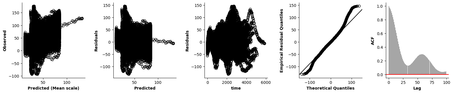
Validation of the assumptions sketched out earlier is absolutely crucial. For the additive model, the independence of \(Y_1\), \(Y_2\), … \(Y_N\) implies that the N-dimensional residual vector (the difference between the observed values \(y_i\) and the model predictions \(\mu_i\)) should look like what could be expected from drawing N independent samples from \(N(0,\sigma)\). This is best checked in residual plots as generated by the plot_val function available from mssmViz. Clearly, this model fails to meet the assumptions - we will get back to that later!!
fig = plt.figure(figsize=(5*single_size,single_size),layout='constrained')
axs = fig.subplots(1,5,gridspec_kw={"wspace":0.1})
plot_val(model,pred_viz=["time"],axs=axs,resid_type="Deviance")
plt.show()
# Of course mssm offers all information visualized in the plots above as attributes/via method calls, so that
# you can also make your own plots. Here some examples:

coef, sigma = model.get_pars() # Coef = weights for basis functions, sigma = **variance** of residuals!
pred = model.preds[0] # The model prediction for the entire data, here: a + f(Time)!
mu = model.mus[0] # The predicted mean - this will be identical to pred for the additive model, but this will not be the case for generalized additive models!
res = model.get_resid() # The residuals y_i - \mu_i
y = model.formulas[0].y_flat[model.formulas[0].NOT_NA_flat] # The dependent variable after NAs were removed
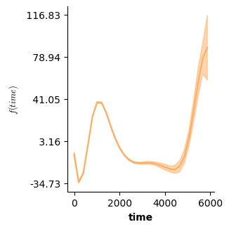
Apart from validation plots, mssmViz also has functions to visualize the model’s estimated smooth terms. Below, we print the estimated smooth of time.
# Plot partial prediction for a single smooth
plot(model,fig_size=(single_size,single_size))
A by-condition GAM
To get a by-factor model (s(Time,by=cond) in mgcv) mssm also provides a by keyword! As mentioned above, by default Formula dummy-codes factor variables in alphapetical order. Hence, for the cond variable “a” will be coded as 0, while “b” will be coded as 1.
# Y = a + b1*c1 + f0(time) + f1(time) + e
# with e ~ N(0,sigma) and c1 == 1 if cond == "b" else 0
# and f0() and f1() representing the smooths over time for
# the first (a) and second (b) level of cond respectively.
formula2 = Formula(lhs=lhs("y"), # The dependent variable - here y!
                        terms=[i(), # The intercept, a
                               l(["cond"]), # One coefficient per dummy-predictor necessary for factor cond - here b
                               f(["time"],by="cond")], # One f(time) term for every level of cond
                        data=dat)
/opt/hostedtoolcache/Python/3.14.3/x64/lib/python3.14/site-packages/mssm/src/python/formula.py:937: UserWarning: 3003 y values (9.32%) are NA.
  warnings.warn(
# Fit the model
model2 = GAMM(formula2,Gaussian())
model2.fit(progress_bar=False)
# Again, we print a summary of the edf. per term in the model.
# Note: separate smooths were estimated for each level of "cond" so two edf values are printed.
model2.print_smooth_terms()
f(['time'],by=cond): a; edf: 6.881
f(['time'],by=cond): b; edf: 8.714
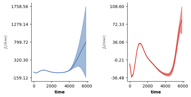
# Partial prediction (using only the f(time)) for all conditions
# Basically what plot(model) does in R in case model was obtained from mgcv
fig = plt.figure(figsize=(2*single_size,single_size),layout='constrained')
axs = fig.subplots(1,2,gridspec_kw={"wspace":0.1})
plot(model2,axs=axs)
plt.show()
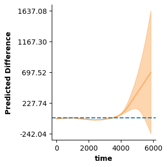
With mssmViz we can also look at the predicted difference in the mean between two conditions: plot_diff allows us to plot the predicted difference over time between conditions a and b. Note that plot_diff does by default take into account all terms included in the model, so the offset differences induced by a and b1 are taken into account!!
You can again use the help or print function, to learn more about the plot_diff function:
print(plot_diff.__doc__)
Plots the expected difference (and CI around this expected difference) between two sets of
predictions, evaluated for `pred_dat1` and `pred_dat2`.

This function works with all GAMM models, but only supports ``GAMMLSS`` and ``GSMM`` models when
setting ``response_scale=False``. The latter is by default set to True, which means that, in
contrast to ``plot``, the predicted difference is computed on the scale of the mean
(i.e., response-scale) by default.

This function is primarily designed to visualize the expected difference between two levels of a
categorical/factor variable. For example, consider the following model below, including a
separate smooth of "time" per level of the factor "cond". It is often of interest to visualize
*when* in time the two levels of "cond" differ from each other in their dependent variable.
For this, the difference curve over "time", essentially the smooth of "time" for the first level
subtracted from the smooth of "time" for the second level of factor "cond" (offset terms can
also be accounted for, check the `use` argument), can be visualized together with a CI
(Wood, 2017). This CI can provide insights into whether and *when* the two levels can be
expected to be different from each other. To visualize this difference curve as well as the
difference CI, this function can be used as follows::

    # Define & estimate model
    model = GAMM(Formula(lhs("y"),[i(), l(["cond"]), f(["time"],by="cond")],data=dat),
        Gaussian())
    model.fit()

    # Create prediction data, differing only in the level of factor cond
    time_pred = np.linspace(0,np.max(dat["time"]),30)
    new_dat1 = pd.DataFrame({"cond":["a" for _ in range(len(time_pred))],
                            "time":time_pred})

    new_dat2 = pd.DataFrame({"cond":["b" for _ in range(len(time_pred))],
                            "time":time_pred})

    # Now visualize diff = (\alpha_a + f_a(time)) - (\alpha_b + f_b(time)) and the CI around
    # diff
    plot_diff(pred_dat1,pred_dat2,["time"],model)

This is only the most basic example to illustrate the usefulness of this function. Many other
options are possible. Consider for example the model below, which allows for
the expected time-course to vary smoothly as a function of additional covariate "x" - achieved
by inclusion of the tensor smooth term of "time" and "x". In addition, this
model allows for the shape of the tensor smooth to differ between the levels of factor "cond"::

    model = GAMM(Formula(lhs("y"),[i(), l(["cond"]), f(["time","x"],by="cond",te=True)],
        data=dat),Gaussian())

For such a model, multiple predicted differences might be of interest. One option would be to
look only at a single level of "cond" and to visualize the predicted difference
in the time-course for two different values of "x" (perhaps two quantiles). In that case,
`pred_dat1` and `pred_dat2` would have to be set up to differ only in the value of
"x" - they should be equivalent in terms of "time" and "cond" values.

Alternatively, it might be of interest to look at the predicted difference between the tensor
smooth surfaces for two levels of factor "cond". Rather than being interested in a difference
curve, this would mean we are interested in a difference *surface*. To achieve this,
`pred_dat1` and `pred_dat2` would again have to be set up to differ only in the value of
"cond" - they should be equivalent in terms of "time" and "x" values. In addition, it would be
necessary to specify `tvars=["time","x"]`. Note that, for such difference surfaces,
areas of the difference prediction for which the CI contains zero will again be visualized with
low opacity if the CI is to be visualized.

References:
 - Wood, S. N. (2017). Generalized Additive Models: An Introduction with R, Second Edition         (2nd ed.).
 - Simpson, G. (2016). Simultaneous intervals for smooths revisited.

:param pred_dat1: A pandas DataFrame containing new data for which the prediction is to be
    compared to the prediction obtained for `pred_dat2`. Importantly, all variables present in
    the data used to fit the model also need to be present in this DataFrame. Additionally,
    factor variables must only include levels also present in the data used to fit the model.
    If you want to exclude a specific factor from the difference prediction (for example the
    factor subject) don't include the terms that involve it in the ``use`` argument.
:type pred_dat1: pandas.DataFrame
:param pred_dat2: Like `pred_dat1` - ideally differing only in the level of a single factor
    variable or the value of a single continuous variable.
:type pred_dat2: pandas.DataFrame
:param tvars: List of variables to be visualized - must contain one string for difference
    predictions visualized as a function of a single variable, two for difference predictions
    visualized as a function of two variables
:type tvars: [str]
:param model: The estimated GAMM or GAMMLSS model for which the visualizations are to be
    obtained
:type model: GAMM or GAMMLSS
:param use: The indices corresponding to the terms that should be used to obtain the prediction
    or ``None`` in which case all fixed effects will be used, defaults to None
:type use: [int]|None, optional
:param dist_par: The index corresponding to the parameter for which to make the prediction
    (e.g., 0 = mean) - only necessary if a GAMMLSS or GSMM model is provided, defaults to 0
:type dist_par: int, optional
:param ci_alpha: The alpha level to use for the standard error calculation. Specifically,
    1 - (``alpha``/2) will be used to determine the critical cut-off value according to a
    N(0,1), defaults to 0.05
:type ci_alpha: float, optional
:param whole_interval: Whether or not to adjuste the point-wise CI to behave like whole-function
    (based on Wood, 2017; section 6.10.2 and Simpson, 2016), defaults to False
:type whole_interval: bool, optional
:param n_ps: How many samples to draw from the posterior in case the point-wise CI is adjusted
    to behave like a whole-function CI, defaults to 10000
:type n_ps: int, optional
:param seed: Can be used to provide a seed for the posterior sampling step in case the
    point-wise CI is adjusted to behave like a whole-function CI, defaults to None
:type seed: int|None, optional
:param cmp: string corresponding to name for a matplotlib colormap, defaults to None in which
    case it will be set to 'RdYlBu_r'.
:type cmp: str|None, optional
:param plot_exist: Whether or not an indication of the data distribution should be provided.
    For difference predictions visualized as a function of a single variable this will simply
    hide predictions outside of the data-limits. For difference predictions visualized as a
    function of a two variables setting this to true will result in values outside of data
    limits being hidden, defaults to False
:type plot_exist: bool, optional
:param response_scale: Whether or not predictions and CIs should be shown on the scale of the
    model predictions (linear scale) or on the 'response-scale' i.e., the scale of the mean,
    defaults to True
:type response_scale: bool, optional
:param ax: A ``matplotlib.axis.Axis`` on which the Figure should be drawn, defaults to None in
    which case an axis will be created by the function and plot.show() will be called at the end
:type ax: matplotlib.axis.Axis, optional
:param fig_size: Tuple holding figure size, which will be used to determine the size of the
    figures created if `ax=None`, defaults to (6/2.54,6/2.54)
:type fig_size: tuple[float,float], optional
:param ylim: Tuple holding y-limits (z-limits for 2d plots), defaults to None in which case
    y_limits will be inferred from the predictions made
:type ylim: tuple[float,float]|None, optional
:param col: A float in [0,1]. Used to get a color for univariate predictions from the chosen
    colormap, defaults to 0.7
:type col: float, optional
:param label: A label to add to the y axis for univariate predictions or to the color-bar for
    tensor predictions, defaults to None
:type label: str|None, optional
:param title: A title to add to the plot defaults to None
:type title: str|None, optional
:param lim_dist: The floating point distance (on normalized scale, i.e., values have to be in
    ``[0,1]``) at which a point is considered too far away from training data. Setting this to
    0 means we visualize only points for which there is trainings data, setting this to 1 means
    visualizing everything. Defaults to 0.1
:type lim_dist: float, optional
:raises ValueError: If a visualization is requested for more than 2 variables
Thus, to visualize the predicted difference we need to set up two data-frames, one per level of “cond”. The plot_diff function then figures out the rest:
time_pred = [t for t in range(0,max(dat["time"]),20)]
new_dat1 = pd.DataFrame({"cond":["a" for _ in range(len(time_pred))],
                         "time":time_pred})

new_dat2 = pd.DataFrame({"cond":["b" for _ in range(len(time_pred))],
                         "time":time_pred})

# Note, by default `plot_diff` excludes predictor ranges for which one of the two conditions
# contains no values (time > 4000 only exists in cond b). This behavior can be changed with
# the `plot_exist` keyword.
fig = plt.figure(figsize=(single_size,single_size),layout='constrained')
ax = fig.subplots(1,1)
plot_diff(new_dat1,new_dat2,["time"],model2,ax=ax)
ax.axhline(0,linestyle='dashed')
plt.show()
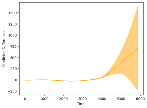
Alternatively, you can also extract the predicted difference yourself, using the model’s predict_diff method and then create your own plot:
pred_diff,b = model2.predict_diff(new_dat1,new_dat2,use_terms=None)


plt.fill([*new_dat1["time"],*np.flip(new_dat1["time"])],
         [*(pred_diff + b),*np.flip(pred_diff - b)],alpha=0.5,color='orange')
plt.plot(new_dat1["time"],pred_diff,color='orange')
plt.xlabel("Time")
plt.ylabel("Predicted Difference")
Text(0, 0.5, 'Predicted Difference')
A binary smooth model
If the difference between conditions is of interest it might be more desirable to directly fit a difference curve for specific levels of the factor of interest, rather than plotting the predicted difference. This can be beneficial in case conditions differ in the values of the predictor over which the difference is to be evaluated, because confidence intervals will often be narrower.
We set up such a model below!
formula3 = Formula(lhs=lhs("y"), # The dependent variable - here y!
                        terms=[i(), # The intercept, a
                               f(["time"]), # One f(time) term - will correspond to the baseline level for condition: here let's choose b
                               f(["time"],binary=["cond","a"])], # Another f(time), this one models the difference over time from the other f(time) term for cond=a!
                        data=dat)
/opt/hostedtoolcache/Python/3.14.3/x64/lib/python3.14/site-packages/mssm/src/python/formula.py:937: UserWarning: 3003 y values (9.32%) are NA.
  warnings.warn(
# Fit the model
model3 = GAMM(formula3,Gaussian())
model3.fit(progress_bar=False)
model3.print_smooth_terms()
f(['time']); edf: 8.72
f(['time'],by=a); edf: 6.693
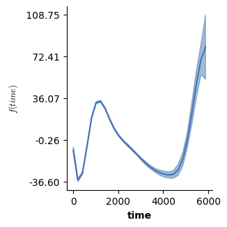
# Let's look at just the f(time) for level b - this one looks just like before!
plot(model3,which=[1],fig_size=(single_size,single_size),prov_cols=0.1)
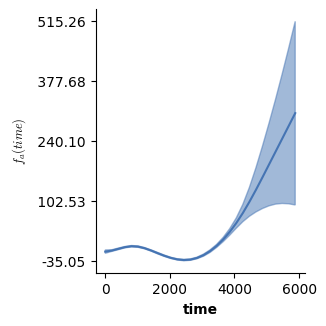
# However, just the prediction from the second f(time) does look a bit different
# now! In fact it represents the difference between the two conditions!
plot(model3,which=[2],fig_size=(single_size,single_size))
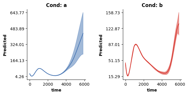
If we use all terms we can still predict how y changes over time for both conditions - and thus essentially recover the predictions from model 2! For this we again make use of the plot_fitted function, which allows to visualize the combined prediction of multiple terms included in the model (again, see the doc string!)
fig = plt.figure(figsize=(2*single_size,single_size),layout='constrained')
axs = fig.subplots(1,2,gridspec_kw={"wspace":0.1})
cols = [0.1,0.9]
titles = ["Cond: a", "Cond: b"]

for ci,c in enumerate(["a","b"]):
    # Set up some new data for prediction
    time_pred = [t for t in range(0,max(dat["time"]),20)]

    new_dat = pd.DataFrame({"cond":[c for _ in range(len(time_pred))],
                            "time":time_pred})

    # Now make prediction using all terms
    plot_fitted(new_dat,["time"],model3,ax=axs[ci],col=cols[ci],use=[0,1,2],title=titles[ci])

plt.show()
An ordered factor model
In mgcv in R, the by keyword is sensitive to whether the factor is of type ordered or not. This is not the case in mssm, but “ordered factor models” can be implemented nonetheless. As mentioned in the previous section, the syntax for the formula is very similar to the binary model - we just need to create an additional “is_by” variable:
dat["is_a"] = (dat["cond"].values == "a").astype(int)

# We also specify a code-book to recode the model so that we get an offset term for level "a" when adding `l(["cond"])` to the model
codebook = {"cond":{"b":0,"a":1}}
formula3O = Formula(lhs=lhs("y"), # The dependent variable - here y!
                        terms=[i(), # The intercept, a
                               l(["cond"]), # An offset term - here for level a
                               f(["time"]), # One f(time) term - will correspond to the baseline level for condition: here let's choose b
                               f(["time"],by_cont="is_a")], # Another f(time), this one models the difference over time from the other f(time) term for cond=a but cannot take on a constant!
                        data=dat,
                        codebook=codebook)
/opt/hostedtoolcache/Python/3.14.3/x64/lib/python3.14/site-packages/mssm/src/python/formula.py:937: UserWarning: 3003 y values (9.32%) are NA.
  warnings.warn(
model3O = GAMM(formula3O,Gaussian())
model3O.fit(progress_bar=False)
model3O.print_parametric_terms()
Intercept: 52.878, t: 211.867, DoF.: 29197, P(|T| > |t|): 0.000e+00 ***
cond_a: -14.002, t: -29.029, DoF.: 29197, P(|T| > |t|): 0.000e+00 ***

Note: p < 0.001: ***, p < 0.01: **, p < 0.05: *, p < 0.1: .
# Let's look at just the f(time) for level b - this one again looks just like before!
plot(model3O,which=[2],fig_size=(single_size,single_size),prov_cols=0.1)
# The predicted effect of the second smooth `f(["time"],by_cont="is_a")`:
plot(model3O,which=[3],fig_size=(single_size,single_size),prov_cols=0.1)
The predicted effect of the second smooth f(["time"],by_cont="is_a") looks very similar to the binary smooth from model 3 - the difference is a different offset shift. To understand what is goind on, remember that both f(["time"],by_cont="is_a") in model 3O and f(["time"],binary=["cond","a"]) in model 3 are difference curves. The distinction is that the latter can include an offset shift, while the former does not. In model 3O, this offset shift is added back in by the l(["cond"]) term:
model3O.print_parametric_terms()
Intercept: 52.878, t: 211.867, DoF.: 29197, P(|T| > |t|): 0.000e+00 ***
cond_a: -14.002, t: -29.029, DoF.: 29197, P(|T| > |t|): 0.000e+00 ***

Note: p < 0.001: ***, p < 0.01: **, p < 0.05: *, p < 0.1: .
If you add -14.002 to the estimate for f(["time"],by_cont="is_a"), you essentially end up again with the estimated effect for f(["time"],binary=["cond","a"]). Note, that while that is true in this simple model, this is not generally the case - depending on how you set up the ordered factor smooths.
Tensor smooth interactions
Non-linear interactions between continuous variables are supported via tensor smooth interactions (see Wood, 2006; Wood, 2017). Both the behavior achieved by the ti() and te() terms in mgcv is supported. Let’s start with considering the te() term behavior!
formula4 = Formula(lhs=lhs("y"), # The dependent variable - here y!
                        terms=[i(), # The intercept, a
                               l(["cond"]), # Offset for cond='b'
                               f(["time","x"],by="cond",te=True)], # one smooth surface over time and x - f(time,x) - per level of cond: three-way interaction!
                        data=dat)
/opt/hostedtoolcache/Python/3.14.3/x64/lib/python3.14/site-packages/mssm/src/python/formula.py:937: UserWarning: 3003 y values (9.32%) are NA.
  warnings.warn(
# Fit the model
model4 = GAMM(formula4,Gaussian())
model4.fit(progress_bar=False)

# We end up with two smooth terms - one surface for every level of cond.
model4.print_smooth_terms()
f(['time', 'x'],by=cond): a; edf: 7.507
f(['time', 'x'],by=cond): b; edf: 8.84
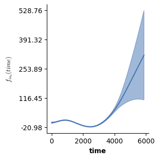
We can now visualize the smooth functions. For this we can again use the plot function. Remember: the plot function only visualizes the estimated smooth terms, it ignores all other terms. That is, in this example the smooth functions are not shifted up/down by the intercept and offset adjustment for level “b” of factor “cond”.
Note: the shaded areas in the plot below correspond to areas outside of a (by default 95%) credible interval.
fig = plt.figure(figsize=(2*single_size,single_size),layout='constrained')
axs = fig.subplots(1,2,gridspec_kw={"wspace":0.3})
plot(model4,axs=axs)
plt.show()
The ti() term in mgcv enables decomposing smooth interactions into separate interaction (including lower order interactions) and main effects! In mssm this is achieved by omitting the te=True argument (the default). In that case, separate smooth terms have to be included for the lower order interactions, just like in mgcv:
formula5 = Formula(lhs=lhs("y"), # The dependent variable - here y!
                        terms=[i(), # The intercept, a
                               l(["cond"]), # Offset for cond='b'
                               f(["time"],by="cond"), # to-way interaction between time and cond; one smooth over time per cond level
                               f(["x"],by="cond"), # to-way interaction between x and cond; one smooth over x per cond level
                               f(["time","x"],by="cond")], # one smooth surface over time and x - f(time,x) - per level of cond: three-way interaction!
                        data=dat)
/opt/hostedtoolcache/Python/3.14.3/x64/lib/python3.14/site-packages/mssm/src/python/formula.py:937: UserWarning: 3003 y values (9.32%) are NA.
  warnings.warn(
# Fit the model
model5 = GAMM(formula5,Gaussian())
model5.fit(progress_bar=False)

# We end up with a total of 6 smooth terms in this model!
model5.print_smooth_terms()
f(['time'],by=cond): a; edf: 6.88
f(['time'],by=cond): b; edf: 8.716
f(['x'],by=cond): a; edf: 1.042
f(['x'],by=cond): b; edf: 1.202
f(['time', 'x'],by=cond): a; edf: 1.0
f(['time', 'x'],by=cond): b; edf: 1.0
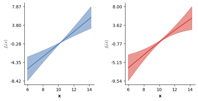
We can now visualize the partial main & interaction effects:
# Visualizing the partial main effects of time.
fig = plt.figure(figsize=(2*single_size,single_size),layout='constrained')
axs = fig.subplots(1,2,gridspec_kw={"wspace":0.1})
plot(model5,which=[2],axs=axs,ci=True)
plt.show()
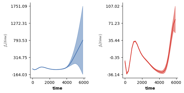
# Visualizing the partial main effects of x.
fig = plt.figure(figsize=(2*single_size,single_size),layout='constrained')
axs = fig.subplots(1,2,gridspec_kw={"wspace":0.1})
plot(model5,which=[3],axs=axs,ci=True)
plt.show()
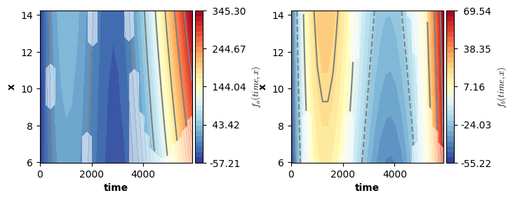
# Visualizing the partial interaction:
fig = plt.figure(figsize=(2*single_size,single_size),layout='constrained')
axs = fig.subplots(1,2,gridspec_kw={"wspace":0.3})
plot(model5,which=[4],axs=axs,ci=False)
plt.show()
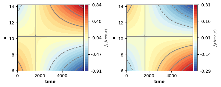
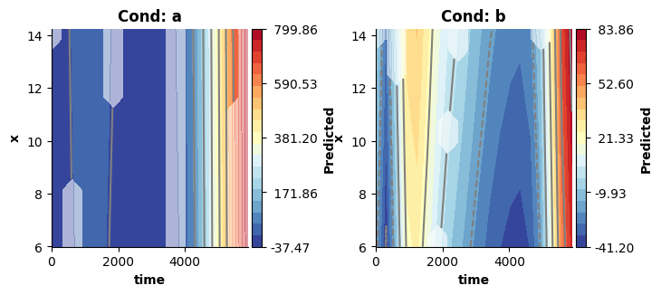
Note, that these surfaces really covers only the three-way interaction estimates (ignoring the main effects). Hence, they look very different from the previous plots. However, we can still recover (approximately) the surfaces estimated by model 4, when visualizing the three-way interaction + the two-way interactions!
In this case, the added interactions produce surfaces comparable to those obtained from model 4. This is not guaranteed, and in practice models set up like model 5 will tend to produce more flexible solutions - because they have a larger solution space, in which they might find evidence for a more complex solution (see Wood, 2017).
# Visualizing the three-way interaction + the two-way interactions approximates the surfaces estimated by model4, which did not attempt to decompose these.
fig = plt.figure(figsize=(2*single_size,single_size),layout='constrained')
axs = fig.subplots(1,2,gridspec_kw={"wspace":0.3})
titles = ["Cond: a", "Cond: b"]

# Set up some new data for prediction
time_pred = []
x_pred = []

xr = [t for t in np.linspace(min(dat["x"]),max(dat["x"]),20)]
tr = np.linspace(0,max(dat["time"]),len(xr))

for t in tr:
    for x in xr:
        time_pred.append(t)
        x_pred.append(x)

# Loop over conditions
for ci,c in enumerate(["a","b"]):


    new_dat = pd.DataFrame({"x":x_pred,
                            "cond":[c for _ in range(len(x_pred))],
                            "time":time_pred})

    plot_fitted(new_dat,["time","x"],model5,ax=axs[ci],use=[2,3,4],title=titles[ci])

plt.show()
Binary tensor smooth interactions
The binary smooth approach generalizes beyond the univariate case to the tensor smooth interaction case. Essentially, we then fit a smooth surface for the reference level and difference surfaces for the remaining levels of a factor. Such a model is set up below.
formula6 = Formula(lhs=lhs("y"), # The dependent variable - here y!
                        terms=[i(), # The intercept, a
                               f(["time","x"],te=True), # one smooth surface over time and x - f(time,x) - for the reference level = cond == b
                               f(["time","x"],te=True,binary=["cond","a"])], # another smooth surface over time and x - f(time,x) - representing the difference from the other surface when cond==a
                        data=dat)
/opt/hostedtoolcache/Python/3.14.3/x64/lib/python3.14/site-packages/mssm/src/python/formula.py:937: UserWarning: 3003 y values (9.32%) are NA.
  warnings.warn(
# Fit the model
model6 = GAMM(formula6,Gaussian())
model6.fit(progress_bar=False)

# We again end up with two smooth terms in the model.
model6.print_smooth_terms()
f(['time', 'x']); edf: 8.499
f(['time', 'x'],by=a); edf: 8.128
Visualizing the two surfaces reveals the same picture visibile for the univariate case: the left surface largely matches the surface estimated by model 4! The right surface is now the difference surface estimated for condition a and thus needs to be added to the surface on the left to get the combined surface for condition a!
fig = plt.figure(figsize=(2*single_size,single_size),layout='constrained')
axs = fig.subplots(1,2,gridspec_kw={"wspace":0.3})
plot(model6,which=[1],axs=[axs[0]],ci=False)
plot(model6,which=[2],axs=[axs[1]],ci=False)
plt.show()
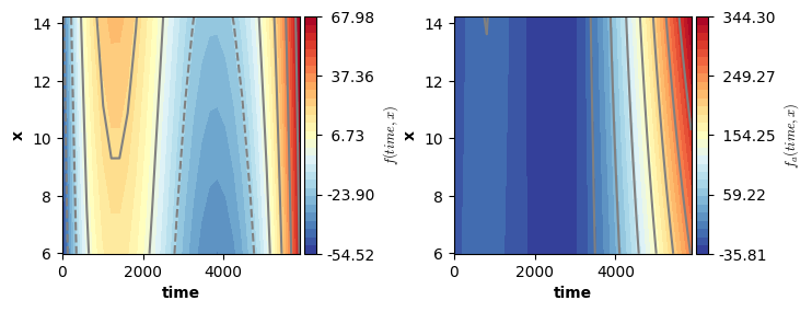
# Hence, to recover the actual surfaces for both conditions we need to add them together when cond == "a"
fig = plt.figure(figsize=(2*single_size,single_size),layout='constrained')
axs = fig.subplots(1,2,gridspec_kw={"wspace":0.3})
titles = ["Cond: a", "Cond: b"]

# Set up some new data for prediction
time_pred = []
x_pred = []

xr = [t for t in np.linspace(min(dat["x"]),max(dat["x"]),20)]
tr = np.linspace(0,max(dat["time"]),len(xr))

for t in tr:
    for x in xr:
        time_pred.append(t)
        x_pred.append(x)

# Loop over conditions
for ci,c in enumerate(["a","b"]):


    new_dat = pd.DataFrame({"x":x_pred,
                            "cond":[c for _ in range(len(x_pred))],
                            "time":time_pred})

    plot_fitted(new_dat,["time","x"],model6,ax=axs[ci],use=[1,2],title=titles[ci],ci=False)

plt.show()
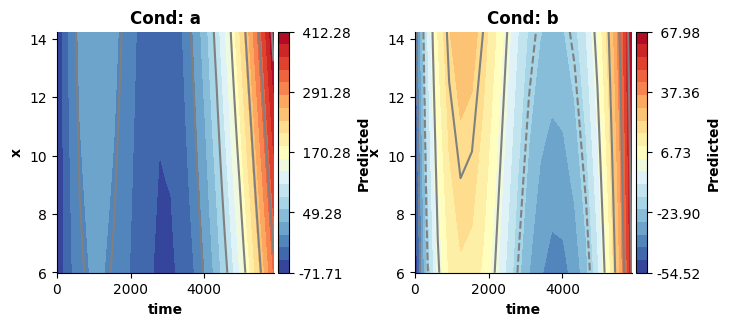
Random effects
As mentioned above we can also include random intercepts, random slopes, and random smooths into any mssm model!
Random Intercepts
To model a random intercept (e.g., per subject or item), simply add an ri term:
formula7a = Formula(lhs=lhs("y"), # The dependent variable - here y!
                        terms=[i(), # The intercept, a
                               l(["cond"]), # For cond='b'
                               f(["time"],by="cond"), # to-way interaction between time and cond; one smooth over time per cond level
                               f(["x"],by="cond"), # to-way interaction between x and cond; one smooth over x per cond level
                               f(["time","x"],by="cond"), # three-way interaction
                               ri("sub")], # Random intercept for each subject
                        data=dat)
/opt/hostedtoolcache/Python/3.14.3/x64/lib/python3.14/site-packages/mssm/src/python/formula.py:937: UserWarning: 3003 y values (9.32%) are NA.
  warnings.warn(
# Fit the model
model7a = GAMM(formula7a,Gaussian())
model7a.fit(progress_bar=False)
model7a.print_smooth_terms()
f(['time'],by=cond): a; edf: 6.906
f(['time'],by=cond): b; edf: 8.753
f(['x'],by=cond): a; edf: 1.0
f(['x'],by=cond): b; edf: 1.074
f(['time', 'x'],by=cond): a; edf: 1.0
f(['time', 'x'],by=cond): b; edf: 1.0
ri(sub); edf: 18.966
You can extract the estimated random intercepts using the get_term_coef function, which returns the coefficients (and their identifiers/names) associated with a specific term in the formula (here term 5, corresponding to the random intercept term):
rand_int,rand_int_names = get_term_coef(model7a,[5])

for ric,rin in zip(rand_int[:5],rand_int_names[:5]):
    print(f"{rin}: {ric[0]}")
ri(sub_0): -22.417954508612798
ri(sub_1): 16.585033688758454
ri(sub_2): -21.772958080652423
ri(sub_3): -0.9703295325880099
ri(sub_4): 4.129825866835075
Random Slopes
Many different random slope combinations are possible - but they are all achieved with the rs term. Check the doc-string for the rs term for different examples. Below
we estimate a random intercept per subject (achieved with the ri term) and also a random slope of time (achieved with the rs term) - with a separate variance parameter per condition:
formula7b = Formula(lhs=lhs("y"), # The dependent variable - here y!
                        terms=[i(), # The intercept, a
                               l(["cond"]), # For cond='b'
                               f(["time"],by="cond"), # to-way interaction between time and cond; one smooth over time per cond level
                               f(["x"],by="cond"), # to-way interaction between x and cond; one smooth over x per cond level
                               f(["time","x"],by="cond"), # three-way interaction
                               ri("sub"), # Random intercept for each subject
                               rs(["time","sub"],by="cond")], # Random slope of time for subject - separate ones for each level of cond
                        data=dat)
# Fit the model
model7b = GAMM(formula7b,Gaussian())
model7b.fit(progress_bar=False)
model7b.print_smooth_terms()
f(['time'],by=cond): a; edf: 6.912
f(['time'],by=cond): b; edf: 8.832
f(['x'],by=cond): a; edf: 1.221
f(['x'],by=cond): b; edf: 1.0
f(['time', 'x'],by=cond): a; edf: 1.0
f(['time', 'x'],by=cond): b; edf: 1.0
ri(sub); edf: 16.826
rs(['time', 'sub'],by=cond):a; edf: 18.869
rs(['time', 'sub'],by=cond):b; edf: 18.913
The get_term_coef function can again be used to obtain the estimated random slopes. Note, that the function returns a single array even though separate sets of random slopes were estimated per level of “cond”: The first 20 (here “sub” had 20 levels, i.e., there were 20 subjects) elements in this array will correspond to the random slopes estimated for the first level of “cond”, the next 20 to the second level, and so on. To check which level of “cond” was treated as the “first level” you can inspect the codebook again, via formula.get_factor_codings().
Since the function also returns the name of each coefficient, you can also inspect those.
rand_slopes,rand_slope_names = get_term_coef(model7b,[6])

for rsc,rsn in zip(rand_slopes[:5],rand_slope_names[:5]):
    print(f"{rsn}: {rsc[0]}")
rs(time_sub_0_a): -0.013782446781860767
rs(time_sub_1_a): 0.00819603584583401
rs(time_sub_2_a): -0.016399453706536456
rs(time_sub_3_a): 0.0013404742623717204
rs(time_sub_4_a): 0.00236796387099529
Random Smooths
GAMMs also allow to decompose the mean into a non-linear fixed part and a non-linear random part - e.g., a general smooth trend over time and factor-level-specific non-linear deviations from it. Additive models estimate the latter as random smooth terms:
formula7c = Formula(lhs=lhs("y"), # The dependent variable - here y!
                        terms=[i(), # The intercept, a
                               l(["cond"]), # For cond='b'
                               f(["time"],by="cond"), # to-way interaction between time and cond; one smooth over time per cond level
                               f(["x"],by="cond"), # to-way interaction between x and cond; one smooth over x per cond level
                               f(["time","x"],by="cond"), # three-way interaction
                               fs(["time"],rf="sub")], # Random smooth for each subject
                        data=dat)
/opt/hostedtoolcache/Python/3.14.3/x64/lib/python3.14/site-packages/mssm/src/python/repara.py:247: FutureWarning: Input has data type int64, but the output has been cast to float64.  In the future, the output data type will match the input. To avoid this warning, set the `dtype` parameter to `None` to have the output dtype match the input, or set it to the desired output data type.
  Srp = scp.sparse.diags(
# Fit the model
model7c = GAMM(formula7c,Gaussian())
model7c.fit(progress_bar=False)
model7c.print_smooth_terms()
f(['time'],by=cond): a; edf: 6.892
f(['time'],by=cond): b; edf: 8.635
f(['x'],by=cond): a; edf: 1.218
f(['x'],by=cond): b; edf: 1.001
f(['time', 'x'],by=cond): a; edf: 1.0
f(['time', 'x'],by=cond): b; edf: 1.001
f(['time'],by=sub); edf: 131.86
# Subject difference smooths - is there a subject-specific difference from the general trend?
plot(model7c,which=[5],fig_size=(single_size,single_size))
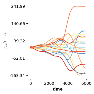
In the R-package mgcv it is common to estimate random smooth terms with separate smoothing penalties for different levels of an additional experimental factor (e.g., cond). In mssm this is achieved with the following syntax (see the conversion table above for an alternative syntax involving the by_cont keyword of fs):
# First we have to create a factor in our data that separates subjects between different levels (i.e., the interaction of the factor cond and sub):
dat["sub_cond"] = dat["cond"].astype(str) + dat["sub"].astype(str)
# Now we can specify the formula:
formula7d = Formula(lhs=lhs("y"), # The dependent variable - here y!
                        terms=[i(), # The intercept, a
                               l(["cond"]), # For cond='b'
                               f(["time"],by="cond"), # to-way interaction between time and cond; one smooth over time per cond level
                               f(["x"],by="cond"), # to-way interaction between x and cond; one smooth over x per cond level
                               f(["time","x"],by="cond"), # three-way interaction
                               fs(["time"],rf="sub_cond",by_subgroup=["cond","a"]), # Random smooth for each subject for group a of factor cond
                               fs(["time"],rf="sub_cond",by_subgroup=["cond","b"])], # Random smooth for each subject for group b of factor cond
                        data=dat)
/opt/hostedtoolcache/Python/3.14.3/x64/lib/python3.14/site-packages/mssm/src/python/formula.py:937: UserWarning: 3003 y values (9.32%) are NA.
  warnings.warn(
/opt/hostedtoolcache/Python/3.14.3/x64/lib/python3.14/site-packages/mssm/src/python/repara.py:247: FutureWarning: Input has data type int64, but the output has been cast to float64.  In the future, the output data type will match the input. To avoid this warning, set the `dtype` parameter to `None` to have the output dtype match the input, or set it to the desired output data type.
  Srp = scp.sparse.diags(
# Fit the model
model7d = GAMM(formula7d,Gaussian())
model7d.fit(progress_bar=False)
model7d.print_smooth_terms()
f(['time'],by=cond): a; edf: 6.894
f(['time'],by=cond): b; edf: 8.523
f(['x'],by=cond): a; edf: 1.069
f(['x'],by=cond): b; edf: 1.069
f(['time', 'x'],by=cond): a; edf: 1.0
f(['time', 'x'],by=cond): b; edf: 1.0
f(['time'],by=sub_cond): a; edf: 87.001
f(['time'],by=sub_cond): b; edf: 134.415
# Now we get to sets of subject difference smooths - one per level of "cond":
plot(model7d,which=[5,6])
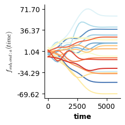
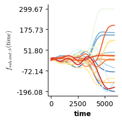
Very big random effect models
mssm is particularly well suited to fit big random effect structures. The model below estimates a non-linear random smooth of time for every individual series in the dataframe - each being parameterized with 20 basis functions.
len(np.unique(dat["series"])) # 200 non-linear curves will be estimated by the random effect.
200
formula9 = Formula(lhs=lhs("y"), # The dependent variable - here y!
                        terms=[i(), # The intercept, a
                               l(["cond"]), # For cond='b'
                               f(["time"],by="cond"), # to-way interaction between time and cond; one smooth over time per cond level
                               f(["x"],by="cond"), # to-way interaction between x and cond; one smooth over x per cond level
                               f(["time","x"],by="cond"), # three-way interaction
                               fs(["time"],rf="series",nk=20)], # Random non-linear effect of time - one smooth per level of factor series
                        data=dat)
/opt/hostedtoolcache/Python/3.14.3/x64/lib/python3.14/site-packages/mssm/src/python/formula.py:937: UserWarning: 3003 y values (9.32%) are NA.
  warnings.warn(
/opt/hostedtoolcache/Python/3.14.3/x64/lib/python3.14/site-packages/mssm/src/python/repara.py:247: FutureWarning: Input has data type int64, but the output has been cast to float64.  In the future, the output data type will match the input. To avoid this warning, set the `dtype` parameter to `None` to have the output dtype match the input, or set it to the desired output data type.
  Srp = scp.sparse.diags(
Note, that we set the method argument to “Chol” in the call to the fit method below. This is slightly less stable than the default QR approach, but usually not problematically so when we have sufficient data. mssm by default will issue a warning if it detects that using the Cholesky approach might result in inaccuracies. In that case you really should switch back to method='QR'.
# Fit the model
model9 = GAMM(formula9,Gaussian())
model9.fit(method="Chol",progress_bar=False)
model9.print_smooth_terms()
f(['time'],by=cond): a; edf: 5.819
f(['time'],by=cond): b; edf: 8.164
f(['x'],by=cond): a; edf: 1.39
f(['x'],by=cond): b; edf: 1.645
f(['time', 'x'],by=cond): a; edf: 1.0
f(['time', 'x'],by=cond): b; edf: 1.211
f(['time'],by=series); edf: 2414.917
# Series difference smooths - is there a series-specific difference from the general trend?
plot(model9,which=[5],fig_size=(single_size,single_size))
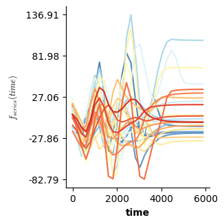
This model finally achieves reasonable model fit - meeting the model assumptions. Note that when modeling multi-level neuro-physiological time-series data in particular it will often be necessary to have trial-level random effect terms to ensure that the assumptions can be met. An “ar1” model is sometimes an alternative, and we will look into that in the “Advanced topics” section!
fig = plt.figure(figsize=(5*single_size,single_size),layout='constrained')
axs = fig.subplots(1,5,gridspec_kw={"wspace":0.1})
plot_val(model9,pred_viz=["time"],axs=axs,resid_type="Deviance")
plt.show()
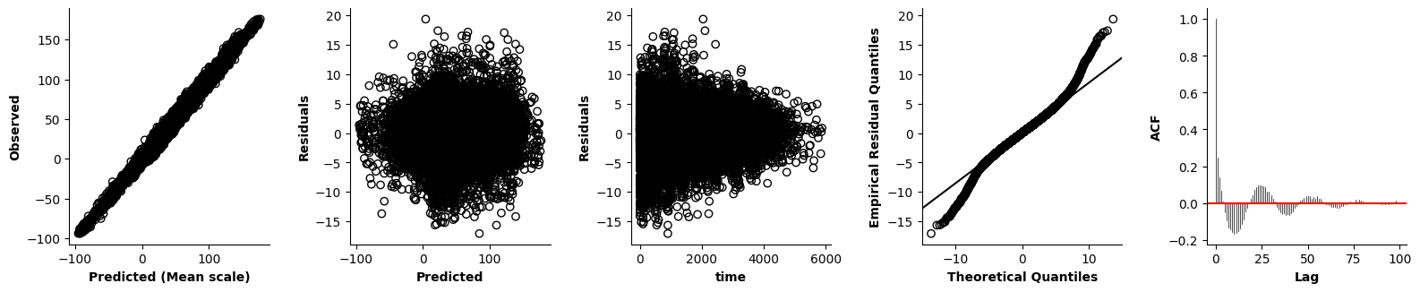
Beyond Gaussian Models: Estimating (Extended) GAMMs and GAMMLSS in mssm
So far we have worked with strictly additive models - this was sufficient to get familiar with the Formula syntax. In a strictly additive model, we assume that our response variables \(Y_i \sim N(\mu_i,\sigma)\), where \(\mu_i\) is the model prediction for observation \(y_i\) (i.e., realization of \(Y_i\)). A Generalized additive model allows to replace the normal distribution with \(\mathcal{E}\) - denoting any member of the exponential family of distributions - so that \(Y_i \sim \mathcal{E}(\mu_i,\phi)\). \(\mu_i\) is usually modelled through a known (link) function \(g(\mu_i) = \eta_i = \mathbf{X}\boldsymbol{\beta}\) with \(\eta_i\) commonly being referred to as the “linear predictor” (since the additive or linear model is specified for \(\eta\)).
mssm currently supports Binomial, Gamma, Inverse Gaussian, and Poisson models. To estimate any non-normal GAMM, all that is necessary in mssm is to replace the Gaussian with any other Family supported by mssm. All families come with default choices for the link functions. You can consult the documentation for details and specific aspects of all families. The documentation also tells you the format expected of response variable. The Binomial family for example assumes that whatever variable is specified as response variable (e.g., “y” in the examples here) - holds observed proportions (of course this will be just 0s and 1s for binary data). Below we present a few examples involving GAMMs with different families. Afterwards we look at GAMMLSS models.
Examples: GAMMs
Binomial GAM
For the implementation of the Binomial family mssm assumes that we have collected proportions of success, i.e., the dependent variables specified in the model Formula needs to hold observed proportions and not counts!
If we assume that each observation \(y_i\) reflects a single independent draw from a binomial, (with \(n=1\), and \(p_i\) being the probability that the result is 1) then the dependent variable should either hold 1 or 0. If we have multiple independent draws from the binomial per observation (i.e., row in our data-frame), then \(n\) will usually differ between observations/rows in our data-frame (i.e., we observe \(k_i\) counts of success out of \(n_i\) draws - so that \(y_i=k_i/n_i\)). In that case, the Binomial() family accepts a vector for argument n (which is simply set to 1 by default, assuming binary data), containing \(n_i\) for every observation \(y_i\).
Below we simulate data for a Binomial GAM:
# Data for Binomial model assumes proportions as DV - for binary this will simply be 0s and 1s.
Binomdat = sim3(10000,2,family=Binomial(),binom_offset=-5,seed=20)
print(Binomdat.head())
print(np.unique(Binomdat["y"],return_counts=True))
   y        x0        x1        x2        x3       eta
0  1  0.280076  0.534054  0.361026  0.625147  4.974914
1  1  0.461147  0.541704  0.534499  0.971402  2.739383
2  1  0.121720  0.763533  0.339944  0.647601  6.633198
3  1  0.522608  0.463200  0.668212  0.994754  2.732701
4  1  0.409168  0.351500  0.372849  0.136747  4.053370
(array([0, 1]), array([2144, 7856]))
Fitting the model should now feel quite familiar - all we need to do is specify a Formula and model. The latter now needs to be set up with the Binomial family.
# Now we can again specify the model.
binom_formula = Formula(lhs("y"),[i(),f(["x0"]),f(["x1"]),f(["x2"]),f(["x3"])],data=Binomdat)

# By default, the Binomial family assumes binary data and uses the logit link.
binom_model = GAMM(binom_formula,Binomial())
binom_model.fit(progress_bar=False)
The plot function from mssmViz continues to function just like before as well. Importantly, the plot function always visualizes effects on the scale of the linear predictor (i.e., here for the log-odds of success). For strictly additive Gaussian models, \(\mu_i = \eta_i\), but this is no longer the case for Generalized models - so keep that in mind for your interpretation of the visualized effects!
# Let's take a look at predictions on the scale of the log-odds
fig = plt.figure(figsize=(4*single_size,single_size),layout='constrained')
axs = fig.subplots(1,4,gridspec_kw={"wspace":0.1})
plot(binom_model,axs=axs)
plt.show()
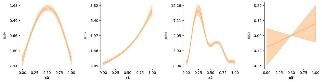
All GAMM functions remain applicable for different families. For example, you can still get p-values for the smooth terms of the Binomial model - but the Null distribution is now automatically adjusted to be a \(\chi^2\) distribution, since no scale parameter is estimated for the Binomial model (see Wood, 2017).
binom_model.print_smooth_terms(p_values=True)
f(['x0']); edf: 4.957 chi^2: 561.981 P(Chi^2 > chi^2) = 0.000e+00 ***
f(['x1']); edf: 4.206 chi^2: 1074.198 P(Chi^2 > chi^2) = 0.000e+00 ***
f(['x2']); edf: 8.712 chi^2: 1327.582 P(Chi^2 > chi^2) = 0.000e+00 ***
f(['x3']); edf: 1.0 chi^2: 1.518 P(Chi^2 > chi^2) = 0.21791

Note: p < 0.001: ***, p < 0.01: **, p < 0.05: *, p < 0.1: . p-values are approximate!
Gamma GAM
Below we simulate data for a Gamma Gam. We assume: \(Y_i \sim \Gamma(\mu_i,\phi)\). The Gamma distribution is usually not expressed in terms of the mean and scale (\(\phi\)) parameter
but rather in terms of a shape and rate parameter - called \(\alpha\) and \(\beta\) respectively. Wood (2017) provides \(\alpha = 1/\phi\). With this we can obtain \(\beta = 1/\phi/\mu\) (see the doc-string for the Gamma family for details).
# Data for Gamma model looks just like for Gaussian - except that y cannot hold negative values!
Gammadat = sim3(500,2,family=Gamma(),seed=0)
print(Gammadat.head())
print(min(Gammadat["y"]))
             y        x0        x1        x2        x3       eta
0    12.379666  0.636962  0.081324  0.013008  0.048017  3.013629
1  2060.005457  0.269787  0.875228  0.827763  0.656338  7.909459
2  5235.301228  0.040974  0.941706  0.496243  0.011885  9.587705
3    68.708860  0.016528  0.261864  0.435918  0.052403  5.189689
4   366.684112  0.813270  0.012101  0.601795  0.023161  5.339632
0.013611044551897237
# Now we can specify the model.
gamma_formula = Formula(lhs("y"),[i(),f(["x0"]),f(["x1"]),f(["x2"]),f(["x3"])],data=Gammadat)

# By default, the Gamma family assumes that the model predictions match log(\mu_i), i.e., a log-link is used.
gamma_model = GAMM(gamma_formula,Gamma())
gamma_model.fit(progress_bar=False)
# Remember: by default the effects are plotted on the scale of the linear predictor - here it is the log of the mean
fig = plt.figure(figsize=(4*single_size,single_size),layout='constrained')
axs = fig.subplots(1,4,gridspec_kw={"wspace":0.1})
plot(gamma_model,axs=axs)
plt.show()
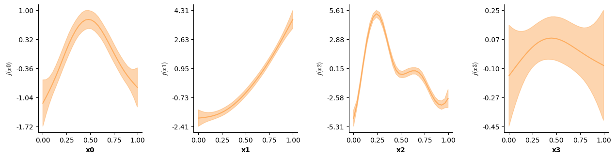
Model validation remains just as crucial for GAMMS as it was for AMMS! We can check the model by inspecting standardized (deviance) residuals (see Wood, 2017 for details) - if the model is correctly specified, we can expect those to behave approximately like \(N(0,\phi)\)!
So the same plots we looked at for the Gaussian model remain relevant - and can again be visualized using the plot_val function from mssmViz.
fig = plt.figure(figsize=(5*single_size,single_size),layout='constrained')
axs = fig.subplots(1,5,gridspec_kw={"wspace":0.1})
plot_val(gamma_model,pred_viz=["x2"],resid_type="Deviance",axs=axs)
plt.show()
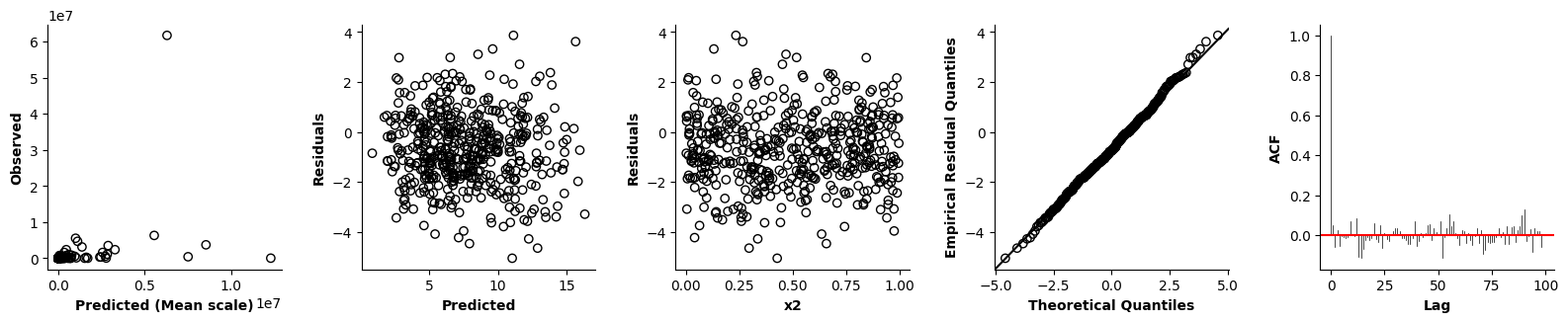
Examples: Extended GAMMs
Sometime, we might want to assume a distribution for the RVs that is not a member of the exponential family or only qualifies as a member when some extra parameters of the likelihood are kept fixed. Specifically, we might want to assume that \(Y_i \sim \mathcal{F}(\mu_i,\phi,...,\tau)\), where \(\mathcal{F}\) denotes some distribution (not necessarily a member of the exponential family) with a likelihood defined by a mean \(\mu_i\) (which is again parameterized by an additive model) and additional parameters \(\phi,...\tau\). This is sometimes referred to as the “extended family” (e.g., Wood et al., 2016).
Such extended models can be estimated like other GAMMs, and mssm currently supports models with a scaled T family where we assume that \((y_i-\mu_i)\phi \sim t_{\nu}\), where \(\nu\) is the degrees of freedom of the t distribution and \(\phi\) acts like a scaling parameter. All that is necessary is to pass an instance of the ExtendedFamily class to the Family argument of the GAMM constructor.
Scaled T GAMMs
Below we re-estimate model 7c, assuming a scaled T distributin for the RVs.
model7cT = GAMM(formula7c,ScaledT(Identity()))
model7cT.fit(progress_bar=False)
model7cT.print_smooth_terms()
f(['time'],by=cond): a; edf: 6.908
f(['time'],by=cond): b; edf: 8.657
f(['x'],by=cond): a; edf: 1.449
f(['x'],by=cond): b; edf: 1.016
f(['time', 'x'],by=cond): a; edf: 1.0
f(['time', 'x'],by=cond): b; edf: 1.014
f(['time'],by=sub); edf: 135.428
All functions that can be used with regular GAMMs continue to function with extended GAMMs. For example, we can again plot the estimated random smooth function. In this case they are virtually indistinguishable from those obtained by model7c assuming a Gaussian family.
plot(model7cT,which=[5],fig_size=(single_size,single_size))
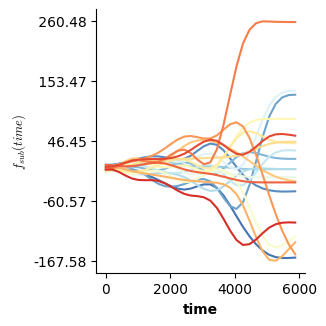
Overall, both models are highly similar. The reason: the best estimate for the degrees of freedom \(\nu\) parameter for the scaled T distribution is a very large number - in which case the scaled t distribution approximates a normal distribution with standard deviation \(\phi\). Any extra parameters of ExtendedFamily models are stored in the family.theta variable and can thus be inspected after estimation. For the scaled t distribution, the first value in theta corresponds to the estimated log scale parameter (e.g., \(\phi\)) while the second value corresponds to the estimated log DoF parameter (e.g., \(\nu\)).
np.exp(model7cT.family.theta)
array([[2.09719015e+01],
       [9.95144450e+57]])
As mentioned since \(\nu\) is a very large value here, the scaled t distribution behaves like a Gaussian with \(\phi\) for the standard deviation - so we can go ahead and compare the obtained estimate for \(\phi\) to the estimate of the standard deviation obtained by model 7c. In this case both estimates are, as would be expected, close:
# Reminder: ``scale`` holds the variance for Gaussian models!
np.sqrt(model7c.scale)
np.float64(24.02490090893369)
Examples: Generalized Additive Models of Location Scale and Shape
(Extended) GAMMs are already more flexible than AMMS and come in handy if we cannot assume that the variance in our RVs \(Y_i\) remains constant. However, they are still quite restrictive in that they restrict the variance to change according to a (often relatively simple) function of the mean of and because they assume that the scale parameter and any other distribution parameter are shared between observations (see Rigby & Stasinopoulos, 2005 for a discussion).
The answer to these problems are Generalized Additive Models of Location, Scale and Shape (GAMMLSS models; Rigby & Stasinopoulos, 2005), in which we model some or even all parameters of the response distributions, not just the mean, as additive combinations of smooth functions and other parametric terms. That is, we assume \(Y_i \sim \mathcal{F}(\mu_i,\phi_i,...,\tau_i)\) For example, in time-series modeling we might assume that our RVs are \(Y_i \sim N(\mu_i,\sigma_i)\) - where both \(\mu_i\) and \(\sigma_i\) change smoothly as a (potentially differently shaped) function of time. Note, that this allows modeling very different patterns of heteroscedasticity - also those that might not easily be captured by modeling the variance as a simple function of the mean.
mssm currently supports Normal models (\(\mu\) and \(\sigma\) can be modelled), Gamma models (\(\mu\) and \(\phi\) can be modeled), and Multinomial models (Probability of \(Y_i\) taking one one of \(K\) values can be modelled).
Gaussian GAMMLSS
Below we simulate data for a Gaussian GAMMLSS model. Both the mean and the standard deviation of \(Y_i\) change as a function of variable x0. Setting up a GAMMLSS model in mssm is not much more work than setting up a GAM. The main difference is that multiple formulas need to be provided - one per distributional parameter of the family.
# Simulate 1000 data points
GAUMLSSDat = sim6(1000,seed=20)

# We need to model the mean: \mu_i = \alpha + f(x0)
formula_m = Formula(lhs("y"),
                    [i(),f(["x0"])],
                     data=GAUMLSSDat)

# and the standard deviation as well: log(\sigma_i) = \alpha + f(x0)
formula_sd = Formula(lhs("y"),
                    [i(),f(["x0"])],
                     data=GAUMLSSDat)

# Collect both formulas
formulas = [formula_m,formula_sd]

# Create Gaussian GAMMLSS family with identity link for mean
# and log link for sigma
family = GAUMLSS([Identity(),LOGb(-0.0001)])

# Now define the model and fit!
gaumlss_model = GAMMLSS(formulas,family)
gaumlss_model.fit(progress_bar=False)
The plot function from the mssmViz package also supports GAMMLSS models, and can be used to visualize the estimated effects for individual distribution parameters (e.g., \(\mu\) and \(\phi\)):
# Now we can visualize the estimated shape of f(x0) for both the mean and standard deviation parameter
# as well as approximate CIs for both.
fig = plt.figure(figsize=(2*single_size,single_size),layout='constrained')
axs = fig.subplots(1,2,gridspec_kw={"wspace":0.1})
plot(gaumlss_model,dist_par=0,axs=[axs[0]])
plot(gaumlss_model,dist_par=1,axs=[axs[1]])
plt.show()
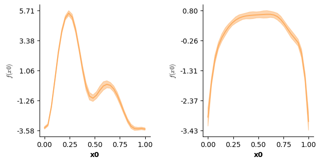
Also for GAMMLSS models we need to check the validity of the model. The plot_val function by default plots standardized residuals for GAMMLSS models - these should be \(N(0,1)\) if the model is correct (see plot_val doc-string and Rigby & Stasinopoulos, 2005):
fig = plt.figure(figsize=(5*single_size,single_size),layout='constrained')
axs = fig.subplots(1,5,gridspec_kw={"wspace":0.1})

# By default, the plot_val function omits the predicted vs. observed plot for more general models - but for Gaussian and Gamma GAMMLSS it is still useful, so we set `obs=True` to get it.
plot_val(gaumlss_model,pred_viz=["x0"],obs=True,axs=axs)
plt.show()
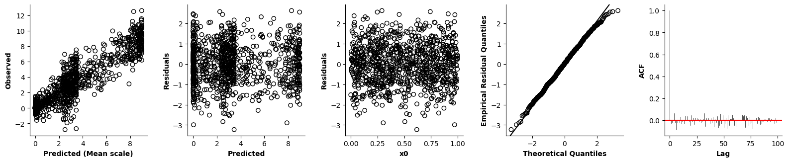
The model presented above is rather simple - but mssm also readily handles more complex GAMMLSS models. Below we simulate a more complex model involving random smooth terms for 20 simulated subjects and then estimate the model from 5000 observations. This only takes a couple of seconds or so.
sim_dat = sim12(5000,c=0,seed=0,family=GAUMLSS([Identity(),LOG()]),n_ranef=20)

# We again need to model the mean: \mu_i = \alpha + f(x0) + f(x1) + f_{x4}(x0)
sim_formula_m = Formula(lhs("y"),
                    [i(),f(["x0"]),f(["x1"]),fs(["x0"],rf="x4")],
                    data=sim_dat)

# and the standard deviation as well: log(\sigma_i) = \alpha + f(x2) + f(x3)
sim_formula_sd = Formula(lhs("y"),
                    [i(),f(["x2"]),f(["x3"])],
                    data=sim_dat)

# Now define the model and fit!
gaumlss_model2 = GAMMLSS([sim_formula_m,sim_formula_sd],family)
gaumlss_model2.fit(progress_bar=False)
/opt/hostedtoolcache/Python/3.14.3/x64/lib/python3.14/site-packages/mssm/src/python/repara.py:247: FutureWarning: Input has data type int64, but the output has been cast to float64.  In the future, the output data type will match the input. To avoid this warning, set the `dtype` parameter to `None` to have the output dtype match the input, or set it to the desired output data type.
  Srp = scp.sparse.diags(
fig = plt.figure(figsize=(5*single_size,single_size),layout='constrained')
axs = fig.subplots(1,5,gridspec_kw={"wspace":0.1})
plot(gaumlss_model2,axs=axs[:3])
plot(gaumlss_model2,axs=axs[3:],dist_par=1)
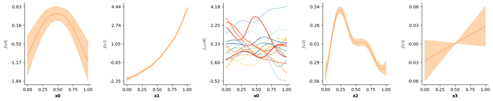
GAMMA GAMMLSS
We now simulate the \(Y_i\) with a Gamma distribution - both mean and scale parameter of the Gamma again vary as a function of x0.
# Simulate 1000 data points
GAMMALSSDat = sim6(1000,family=GAMMALS([LOG(),LOG()]),seed=20)

# We need to model the mean: \mu_i = \alpha + f(x0)
formula_m = Formula(lhs("y"),
                    [i(),f(["x0"])],
                     data=GAMMALSSDat)

# and the scale parameter as well: log(\scale_i) = \alpha + f(x0)
formula_sd = Formula(lhs("y"),
                    [i(),f(["x0"])],
                     data=GAMMALSSDat)

# Collect both formulas
formulas = [formula_m,formula_sd]

# Create Gamma GAMMLSS family with log link for mean
# and log link for sigma
family = GAMMALS([LOG(),LOGb(-0.01)])

# Now define the model and fit!
gammalss_model = GAMMLSS(formulas,family)
gammalss_model.fit(progress_bar=False)
# Now we can again visualize the estimated shape of f(x0) for both the mean and scale parameter
# as well as approximate CIs for both.
fig = plt.figure(figsize=(2*single_size,single_size),layout='constrained')
axs = fig.subplots(1,2,gridspec_kw={"wspace":0.1})
plot(gammalss_model,dist_par=0,axs=[axs[0]])
plot(gammalss_model,dist_par=1,axs=[axs[1]])
plt.show()
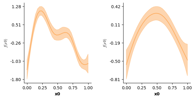
Multinomial GAMMLSS
The final GAMMLSS example is for a multinomial model. This Family assumes that each observation \(y_i\) corresponds to one of \(K\) classes (labeled as 0,…,\(K\)) and reflects a realization of an independent RV \(Y_i\) with probability mass function defined over the \(K\) classes. These K probabilities - that \(Y_i\) takes on class 0,…,\(K\) - are modeled as additive combinations of smooth functions of covariates and other parametric terms. This model can thus be used to perform multi-label classification!
Below we simulate for a Multinomial model with 5 classes - with the probability of \(Y_i\) taking on any of these classes changing as a function of variable X0.
# Simulate data
MULNOMDAT = sim5(1000,seed=34)

# We need to specify K-1 formulas - see the `MULNOMLSS` docstring for details.
formulas = [Formula(lhs("y"),
                    [i(),f(["x0"])],
                     data=MULNOMDAT) for k in range(4)]

# Create family - again specifying K-1 pars - here 4!
family = MULNOMLSS(4)

# Fit the model
model = GAMMLSS(formulas,family)
model.fit(method="QR/Chol",progress_bar=False)
# The plot function can again be used to visualize the estimated effects on the scale of the linear predictor.
fig = plt.figure(figsize=(4*single_size,single_size),layout='constrained')
axs = fig.subplots(1,4,gridspec_kw={"wspace":0.1})
plot(model,dist_par=0,axs=[axs[0]])
plot(model,dist_par=1,axs=[axs[1]])
plot(model,dist_par=2,axs=[axs[2]])
plot(model,dist_par=3,axs=[axs[3]])
plt.show()
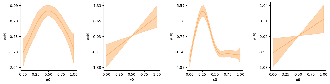
# Visualizing how the probability of Y_i taking on any of the K=5 values is a bit
# more complicated. However, the code below outlines how to achieve this.

# First obtain the K-1 model predictions
pred_dat = pd.DataFrame({"x0":np.linspace(0,1,30)})
mus = []
for k in range(4):

    eta,_,_ = model.predict([0,1],pred_dat,ci=False,par=k)
    mu = family.links[k].fi(eta)
    mus.append(mu)

# These can now be transformed into the K class probabilities (see the MULNOMLSS methods doc-strings for details):
mu_first = np.sum(mus,axis=0) + 1
mus = [mu/mu_first for mu in mus]
mus.insert(0,1/mu_first)

# Now we can plot the K class probabilities as a function of X0:
for k in range(5):
    plt.plot(pred_dat['x0'],mus[k],label=f"Class: {k}")
plt.legend()
plt.xlabel("x0",fontweight='bold')
plt.ylabel("P(Y = class k)",fontweight='bold')
plt.show()
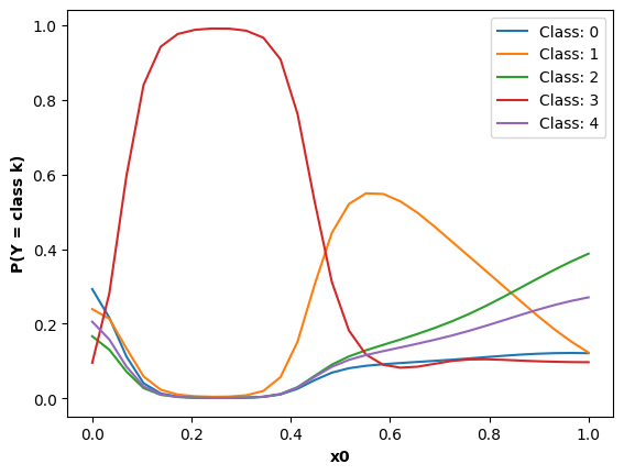
Advanced topics
In this section we discuss advanced use-cases of mssm. We start with an overview of how model selection can be achieved.
Model selection
mssm supports penalty-based model selection (see; Marra & Wood, 2011). In practice, that means the models can penalize entire terms out of the model (they become ~ equal to zero over their covariate(s)). To enable this, provide the penalize_null=True argument to splines for which this should be enabled.
Note: using this with anova-like smooth interactions can result to weird situations, where the marginals are (partially) penalized away but not the (higher-order) partial interaction effects. This can complicate interpretation.
This selection method is particularly efficient for large models, involving many (random) terms. We demonstrate this using the example model considered previously, featuring series-specific random smooth terms:
formula10 = Formula(lhs=lhs("y"), # The dependent variable - here y!
                        terms=[i(), # The intercept, a
                               l(["cond"]), # For cond='b'
                               f(["time"],by="cond"), # two-way interaction between time and cond; one smooth over time per cond level
                               f(["x"],by="cond",penalize_null=True), # two-way interaction between x and cond; one smooth over x per cond level
                               f(["time","x"],by="cond",penalize_null=True), # three-way interaction
                               fs(["time"],rf="series",nk=20)], # Random non-linear effect of time - one smooth per level of factor series
                        data=dat)
/opt/hostedtoolcache/Python/3.14.3/x64/lib/python3.14/site-packages/mssm/src/python/formula.py:937: UserWarning: 3003 y values (9.32%) are NA.
  warnings.warn(
/opt/hostedtoolcache/Python/3.14.3/x64/lib/python3.14/site-packages/mssm/src/python/repara.py:247: FutureWarning: Input has data type int64, but the output has been cast to float64.  In the future, the output data type will match the input. To avoid this warning, set the `dtype` parameter to `None` to have the output dtype match the input, or set it to the desired output data type.
  Srp = scp.sparse.diags(
# Fit the model
model10 = GAMM(formula10,Gaussian())
model10.fit(method="Chol",progress_bar=False)
model10.print_smooth_terms()
f(['time'],by=cond): a; edf: 5.819
f(['time'],by=cond): b; edf: 8.164
f(['x'],by=cond): a; edf: 1.489
f(['x'],by=cond): b; edf: 1.581
f(['time', 'x'],by=cond): a; edf: 0.0 *
f(['time', 'x'],by=cond): b; edf: 0.0 *
f(['time'],by=series); edf: 2414.935

2 terms have been effectively penalized to zero and are marked with a '*'
A non-linear two-way interaction between time and x is not supported for any level of the factor cond (since the edf for the two-way interactions are close to 0).
This is also supported by confidence intervals for the two-way interaction: The confidence intervals for the partial two-way interaction effects contain zero for every x and time combination:
fig = plt.figure(figsize=(2*single_size,single_size),layout='constrained')
axs = fig.subplots(1,2,gridspec_kw={"wspace":0.3})
plot(model10,which=[4],axs=axs,ci=True)
plt.show()
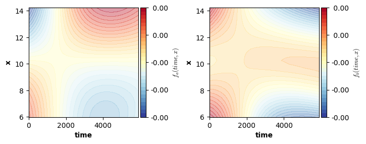
This suggests that we might get away with dropping the partial two-way interactions of time and x for both levels of factor cond. However, we might want to check first how a model involving only two-way interactions performs against this three-way interaction model. This would be a nested comparison, differing only in a single term we want to check for (the partial three-way interaction). For this we can rely on an approximate GLRT or AIC (see Wood 2017), to check whether the reduction in complexity leads to a drastically worse fit.
Note, the GLRT should not be combined with penalty-based selection. Hence, model 10 needs to be re-estimated without an extra Kernel penalty.
formula10 = Formula(lhs=lhs("y"), # The dependent variable - here y!
                        terms=[i(), # The intercept, a
                               l(["cond"]), # For cond='b'
                               f(["time"],by="cond"), # two-way interaction between time and cond; one smooth over time per cond level
                               f(["x"],by="cond"), # two-way interaction between x and cond; one smooth over x per cond level
                               f(["time","x"],by="cond"), # three-way interaction
                               fs(["time"],rf="series",nk=20)], # Random non-linear effect of time - one smooth per level of factor series
                        data=dat)

formula11 = Formula(lhs=lhs("y"), # The dependent variable - here y!
                        terms=[i(), # The intercept, a
                               l(["cond"]), # For cond='b'
                               f(["time"],by="cond"), # two-way interaction between time and cond; one smooth over time per cond level
                               f(["x"],by="cond"), # two-way interaction between x and cond; one smooth over x per cond level
                               f(["time","x"]), # two-way interaction between x and time
                               fs(["time"],rf="series",nk=20)], # Random non-linear effect of time - one smooth per level of factor series
                        data=dat)
/opt/hostedtoolcache/Python/3.14.3/x64/lib/python3.14/site-packages/mssm/src/python/formula.py:937: UserWarning: 3003 y values (9.32%) are NA.
  warnings.warn(
/opt/hostedtoolcache/Python/3.14.3/x64/lib/python3.14/site-packages/mssm/src/python/repara.py:247: FutureWarning: Input has data type int64, but the output has been cast to float64.  In the future, the output data type will match the input. To avoid this warning, set the `dtype` parameter to `None` to have the output dtype match the input, or set it to the desired output data type.
  Srp = scp.sparse.diags(
# Fit the models
model10 = GAMM(formula10,Gaussian())
model10.fit(method="Chol",progress_bar=False)
model10.print_smooth_terms()

model11 = GAMM(formula11,Gaussian())
model11.fit(method="Chol",progress_bar=False)
model11.print_smooth_terms()
f(['time'],by=cond): a; edf: 5.819
f(['time'],by=cond): b; edf: 8.164
f(['x'],by=cond): a; edf: 1.39
f(['x'],by=cond): b; edf: 1.645
f(['time', 'x'],by=cond): a; edf: 1.0
f(['time', 'x'],by=cond): b; edf: 1.211
f(['time'],by=series); edf: 2414.917
f(['time'],by=cond): a; edf: 5.819
f(['time'],by=cond): b; edf: 8.164
f(['x'],by=cond): a; edf: 1.424
f(['x'],by=cond): b; edf: 1.537
f(['time', 'x']); edf: 1.0
f(['time'],by=series); edf: 2414.927
CDL_res = compare_CDL(model10,model11,perform_GLRT=True)
print(f"Accepting alternative hypothesis that the two-way interaction between time and x actually differs between cond levels? {CDL_res['H1'] == 1}")
print(f"Probability of observing twice the difference in log-likelihood as extreme or more extreme than {CDL_res['test_stat']}\nunder the Null (interaction between time and x does not differ between cond levels): {CDL_res['p']}")
print(f"AIC difference between model 1 and model 2: {CDL_res['aic_diff']}")
Accepting alternative hypothesis that the two-way interaction between time and x actually differs between cond levels? False
Probability of observing twice the difference in log-likelihood as extreme or more extreme than 0.8714114990143571
under the Null (interaction between time and x does not differ between cond levels): 0.9721959955220107
AIC difference between model 1 and model 2: 8.7360023194924
In this case the GLRT would also suggest that the three-way interaction does not contribute significantly to the model. Similarly, the strongly positive AIC difference indicates that model 1, the one including the three-way interaction, does not provide a much better fit. Hence, model 11 (including only the two-way interactions) is probably just as good a model as model 10. Importantly, the GLRT test and AIC criterion are both biased and not necessarily conservative enough - in particular when setting correct_V=False (see Wood, Pya, & Säfken; 2016, Smoothing Parameter and Model Selection for General Smooth Models.).
In practice, it should always be set to True (the default - note, that there are many strategies available to correct for the bias, mssm will automatically select an appropriate one based on the specific model passed to the compare_CDL function). See the doc-string for compare_CDL for more details and consult the references therein. However, even with correct_V=True it is generally true that:
In practice, the test should generally be combined with other evidence (i.e., based on null-penalty information or confidence intervals). p-values close to one’s personal alpha level should be considered very carefully.
Finally, note that the compare_CDL function works with GAMMLSS and GSMM models as well. Below we show another example demonstrating model selection for a GAMMLSS model.
# Simulate some data - effect of f0 is zero everywhere!
sim_fit_dat = sim3(n=500,scale=2,c=0,family=Gamma(),seed=21)

# Now fit first model - with f0
sim_fit_formula = Formula(lhs("y"),
                            [i(),f(["x0"]),f(["x1"]),f(["x2"]),f(["x3"])],
                            data=sim_fit_dat,
                            print_warn=False)

sim_fit_formula_sd = Formula(lhs("y"),
                            [i()],
                            data=sim_fit_dat,
                            print_warn=False)

sim_fit_model = GAMMLSS([sim_fit_formula,copy.deepcopy(sim_fit_formula_sd)],family = GAMMALS([LOG(),LOGb(-0.001)]))
sim_fit_model.fit(progress_bar=False)
Now, we know that there is actually no effect of f(["x0"]) in this data. How can we test for this? One option is to start by looking at the estimated effect and confidence intervals:
fig = plt.figure(figsize=(4*single_size,single_size),layout='constrained')
axs = fig.subplots(1,4,gridspec_kw={"wspace":0.1})
plot(sim_fit_model,axs=axs)
axs[0].axhline(0)
<matplotlib.lines.Line2D at 0x7f309a175400>
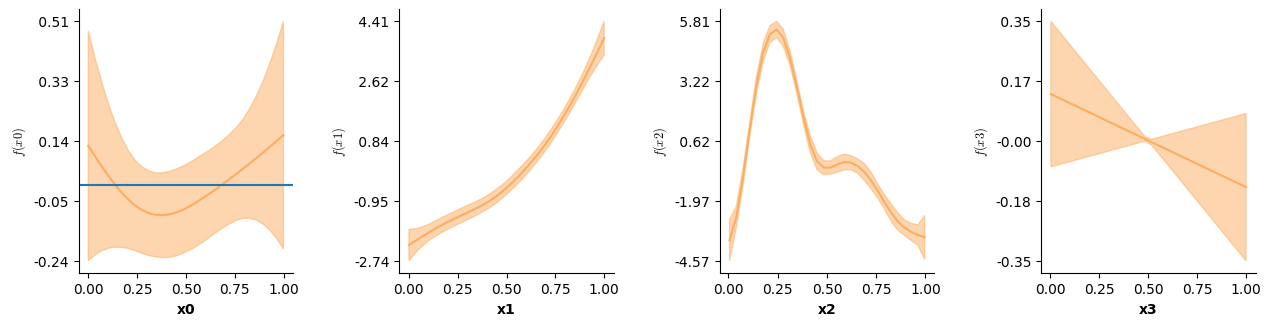
Now, the CI for f(["x0"]) clearly includes zero for every value of the covariate - suggesting that there is no effect of “x0”. We can also extract a p-value for this via the
print_smooth_terms function:
sim_fit_model.print_smooth_terms(p_values=True)
Distribution parameter: 1

f(['x0']); edf: 1.908 chi^2: 2.345 P(Chi^2 > chi^2) = 0.49714
f(['x1']); edf: 3.46 chi^2: 643.143 P(Chi^2 > chi^2) = 0.000e+00 ***
f(['x2']); edf: 8.075 chi^2: 1521.754 P(Chi^2 > chi^2) = 0.000e+00 ***
f(['x3']); edf: 1.0 chi^2: 1.551 P(Chi^2 > chi^2) = 0.21295

Note: p < 0.001: ***, p < 0.01: **, p < 0.05: *, p < 0.1: . p-values are approximate!

Distribution parameter: 2


Note: p < 0.001: ***, p < 0.01: **, p < 0.05: *, p < 0.1: . p-values are approximate!
This also suggests that the effect of f(["x0"]) is unlikely to be significantly different from zero at any point of the covariate (p = 0.21331). As an alternative, we can again rely on an approximate GLRT or AIC. For this we first need to fit a nested model again, excluding f(["x0"]):
# Fit a nested model - without f0:
sim_fit_formula2 = Formula(lhs("y"),
                            [i(),f(["x1"]),f(["x2"]),f(["x3"])],
                            data=sim_fit_dat,
                            print_warn=False)

sim_fit_model2 = GAMMLSS([sim_fit_formula2,copy.deepcopy(sim_fit_formula_sd)],family = GAMMALS([LOG(),LOGb(-0.001)]))
sim_fit_model2.fit(progress_bar=False)
Now we can again use the compare_CDL function:
CDL_res = compare_CDL(sim_fit_model,sim_fit_model2,perform_GLRT=True)
print(f"Accepting alternative hypothesis that the f(['x0']) term is not zero everywhere? {CDL_res['H1'] == 1}")
print(f"Probability of observing twice the difference in log-likelihood as extreme or more extreme than {CDL_res['test_stat']}\nunder the Null (the f(['x0']) term is zero everywhere): {CDL_res['p']}")
print(f"AIC difference between model 1 and model 2: {CDL_res['aic_diff']}")
Accepting alternative hypothesis that the f(['x0']) term is not zero everywhere? False
Probability of observing twice the difference in log-likelihood as extreme or more extreme than 2.493890206692413
under the Null (the f(['x0']) term is zero everywhere): 0.4874547398843416
AIC difference between model 1 and model 2: 2.695374907776568
Again, neither the GLRT nor the AIC score of ~ 2.6351 suggest that we need to include f(["x0"]). Hence, the second model excluding it should be preferred.
Very big random effect models
mssm can approximate the computations involved in determining the smoothness penalty for trial/series-level random smooth terms for Gaussian additive models. This can drastically speed up the time it takes to fit the model. Below, we demonstrate this by re-estimating model 9. Note, that the approximate model might differ slightly in terms of edf and fitted effects from the exact model.
Approximating computations requires specifying a discretization dictionary for each random smooth term for which computations should be approximate. The dictionary must implement this structure: {"no_disc":[str],"excl":[str],"split_by":[str],"restarts":int}:
no_discshould usually be set to an empty list, and should in general only contain names of continuous variables included in the formula. Any variable included in this list will not be discretized in advance. This can improve performance if continuous variables are included with less than 10 unique values. However, it also slows down the clustering that is performed as part of the approximation strategy.Similarly,
exclspecifies any continuous variables that should be excluded for clustering - this can speed up clustering quite a bit but the resulting model might differ more from the exact one because variables are essentially ignored for the computation. Hence, this should only be set to an non-empty list if you really know what you are doing.split_byshould generally be set to a list containing all categorical variables present in the formula.restartsindicates the number of times to re-produce the clustering (should be set to at least 40). Increasing this number usually leads to better results - but the upfront computation cost is increased.
# Approximating computations requires specifying a discretization dictionary.
discretize = {"no_disc":[],"excl":[],"split_by":["cond"],"restarts":40, "seed":20}

formula12 = Formula(lhs=lhs("y"),
                        terms=[i(),
                               l(["cond"]),
                               f(["time"],by="cond"),
                               f(["x"],by="cond"),
                               f(["time","x"],by="cond"),
                               fs(["time"],rf="series",nk=20,approx_deriv=discretize)],
                        data=dat,
                        print_warn=False,
                        series_id="series") # When approximating the computations for a random smooth, the series identifier column needs to be specified!
/opt/hostedtoolcache/Python/3.14.3/x64/lib/python3.14/site-packages/mssm/src/python/repara.py:247: FutureWarning: Input has data type int64, but the output has been cast to float64.  In the future, the output data type will match the input. To avoid this warning, set the `dtype` parameter to `None` to have the output dtype match the input, or set it to the desired output data type.
  Srp = scp.sparse.diags(
# Fit the model
model12 = GAMM(formula12,Gaussian())
model12.fit(method="Chol",progress_bar=False)
model12.print_smooth_terms()
f(['time'],by=cond): a; edf: 5.824
f(['time'],by=cond): b; edf: 8.164
f(['x'],by=cond): a; edf: 1.389
f(['x'],by=cond): b; edf: 1.645
f(['time', 'x'],by=cond): a; edf: 1.0
f(['time', 'x'],by=cond): b; edf: 1.21
f(['time'],by=series); edf: 2432.153
Very big random effect models + MANY observations
In case a Gaussian model needs to be estimated with a big random effect structure and from more than 3-4 million observations, mssm can follow the strategy described in “Generalized additive models for large data sets” (Wood, Goude, and Shaw; 2015) to only build the products involving the model matrix once and to never accumulate the entire model matrix. This requires that the data-set is separated into multiple smaller .csv files (see the code below for an example split of the sim_dat.csv) - which mssm will process in parallel to accumulate the products involving the model matrix.
At every iteration the model predictions need to be obtained which requires the product of a row-block of the model matrix and the current estimate of the coefficient vector. mssm either needs to re-compute the row-block for each prediction or can rely on caching to read it from a drive. For extremely big models (> 20 million observations) the latter can be substantially faster (depending on the system’s hardware). By default caching is disabled. To enable it the mssm.src.python.gamm_solvers.SHOULD_CACHE variable should be set to True. The mssm.src.python.gamm_solvers.CACHE_DIR variable determines the relative location (default “./.db”) of the cache directory. The directory will be deleted after estimation (if running the model fails, the directory might persist - mssm will require the user to manually delete the directory in that case).
Below we re-estimate model 10 (with the extra Kernel penalties) using this iterative building strategy. In terms of fit and edf both models should be viertually identical.
# Note: Categorical variables need to be stored in a way that makes it obvious to pandas that they are not numeric.
# The code below shows how the data for this example were split

if False:
    for cond in np.unique(dat["cond"]):
        cond_dat = dat.loc[dat["cond"] == cond,:]
        cond_dat.loc[:,"series"] = "series_" + cond_dat["series"].astype(str)
        cond_dat.loc[:,"sub"] = "sub_" + cond_dat["sub"].astype(str)

        cond_dat.to_csv(f"./data/GAMM/sim_dat_cond_{cond}.csv",index=False,header=True)
# Now we just collect the paths to the split files and pass those to the formula.
file_paths = [f'https://raw.githubusercontent.com/JoKra1/mssmViz/main/data/GAMM/sim_dat_cond_{cond}.csv' for cond in ["a","b"]]
import mssm as mssm

# Disable caching (default)
mssm.src.python.gamm_solvers.SHOULD_CACHE = False

# Ensure ordering matches the one enforced automatically for model11.
codebook = {'cond':{'a': 0, 'b': 1}}

formula13 = Formula(lhs=lhs("y"),
                        terms=[i(),
                               l(["cond"]),
                               f(["time"],by="cond"),
                               f(["x"],by="cond",penalize_null=True),
                               f(["time","x"],by="cond",penalize_null=True),
                               fs(["time"],rf="series",nk=20)],
                        data=None, # No data frame!
                        file_paths=file_paths, # Just a list with paths to files.
                        print_warn=False,
                        keep_cov=False, # Re-read and encode all data from file at every iteration - further reducing memory footprint, but can slow down if reading takes long
                        codebook=codebook,
                        file_loading_nc = 10) # Set number of cores used for building X.TX in parallel!
# Fit the model
model13 = GAMM(formula13,Gaussian())
model13.fit(method="Chol",progress_bar=False)
model13.print_smooth_terms()
f(['time'],by=cond): a; edf: 5.819
f(['time'],by=cond): b; edf: 8.164
f(['x'],by=cond): a; edf: 1.489
f(['x'],by=cond): b; edf: 1.581
f(['time', 'x'],by=cond): a; edf: 0.0 *
f(['time', 'x'],by=cond): b; edf: 0.0 *
f(['time'],by=series); edf: 2414.935

2 terms have been effectively penalized to zero and are marked with a '*'
You can also combine the iterative model building with the derivative approximation strategy. Note, that this only works with keep_cov=True:
discretize = {"no_disc":[],"excl":[],"split_by":["cond"],"restarts":40, "seed":20}

formula13d = Formula(lhs=lhs("y"),
                        terms=[i(),
                               l(["cond"]),
                               f(["time"],by="cond"),
                               f(["x"],by="cond",penalize_null=True),
                               f(["time","x"],by="cond",penalize_null=True),
                               fs(["time"],rf="series",nk=20,approx_deriv=discretize)],
                        data=None, # Still no data frame!
                        file_paths=file_paths, # Still just a list with paths to files.
                        print_warn=False,
                        keep_cov=True, # Cannot re-read and encode all data from file at every iteration when also relying on the deriv. approx. strategy
                        codebook=codebook,
                        file_loading_nc = 10,
                        series_id="series") # When approximating the computations for a random smooth, the series identifier column needs to be specified!
# Fit the model
model13d = GAMM(formula13d,Gaussian())
model13d.fit(method="Chol",progress_bar=False)
model13d.print_smooth_terms()
f(['time'],by=cond): a; edf: 5.829
f(['time'],by=cond): b; edf: 8.164
f(['x'],by=cond): a; edf: 1.487
f(['x'],by=cond): b; edf: 1.58
f(['time', 'x'],by=cond): a; edf: 0.0 *
f(['time', 'x'],by=cond): b; edf: 0.0 *
f(['time'],by=series); edf: 2451.662

2 terms have been effectively penalized to zero and are marked with a '*'
ar1 Models of the residuals
Fitting series-specific random smooth terms will get expensive the more series collected - even using the tricks discussed above. In addition, including this many coefficients is not really justified for Generalized models (see Wood et al., 2015 for a discussion). An alternative is to specify an “ar1” model of the residuals - capturing dependencies between residuals based on a first-order auto-regressive model (see Wood et al., 2015 and Wood, 2017 for an introduction).
Below, we show how to set up an “ar1” model in mssm. To understand the need for an “ar1” model, consider model 7d. This model was already quite complex - including subject-specific random smooth terms, separately per level of factor “cond”:
model7d.print_smooth_terms()
f(['time'],by=cond): a; edf: 6.894
f(['time'],by=cond): b; edf: 8.523
f(['x'],by=cond): a; edf: 1.069
f(['x'],by=cond): b; edf: 1.069
f(['time', 'x'],by=cond): a; edf: 1.0
f(['time', 'x'],by=cond): b; edf: 1.0
f(['time'],by=sub_cond): a; edf: 87.001
f(['time'],by=sub_cond): b; edf: 134.415
Still, the residuals clearly show remaining dependencies that the model does not account for:
fig = plt.figure(figsize=(5*single_size,single_size),layout='constrained')
axs = fig.subplots(1,5,gridspec_kw={"wspace":0.1})
plot_val(model7d,resid_type="Pearson",pred_viz=["time"],axs=axs)
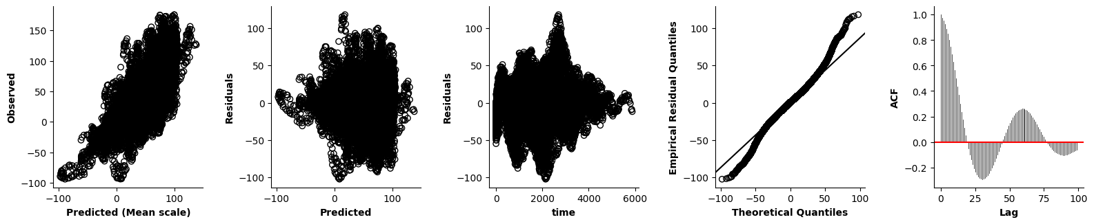
Now, we can try and use an “ar1” model to account for these dependencies. Note, that we should set up the “ar1” model in such a way, that the model restarts with every collected time-series and does not treat the entire residual series as one long time-series. To achieve this, we need to specify the series_id argument, when setting up the formula of the model (see the code examples of the Formula class for more details):
# Now we can specify the formula:
formula7d_ar = Formula(lhs=lhs("y"),
                        terms=[i(),
                               l(["cond"]),
                               f(["time"],by="cond"),
                               f(["x"],by="cond"),
                               f(["time","x"],by="cond"),
                               fs(["time"],rf="sub_cond",by_subgroup=["cond","a"]),
                               fs(["time"],rf="sub_cond",by_subgroup=["cond","b"])],
                        data=dat,
                        series_id="series") # Setting series_id to a string instead of None means the 'ar1' model will restart per series!
/opt/hostedtoolcache/Python/3.14.3/x64/lib/python3.14/site-packages/mssm/src/python/formula.py:937: UserWarning: 3003 y values (9.32%) are NA.
  warnings.warn(
Now, specifying the model works just as before. The difference, is that we now need to set the rho argument of the model.fit method. rho has to be set to the weight of the auto-regressive parameter. A good starting point is to pick the absolute value of the auto-correlation at lag 1 of model 7d, which is approximately 0.98 here:
model7d_ar = GAMM(formula7d_ar,Gaussian())
model7d_ar.fit(rho=0.97,progress_bar=False)
Now, we can compare the “ar1-corrected” residuals (see Wood, 2017) of this model, to the residuals of the previous model:
fig = plt.figure(figsize=(5*single_size,single_size),layout='constrained')
axs = fig.subplots(1,5,gridspec_kw={"wspace":0.1})
plot_val(model7d_ar,resid_type="ar1",pred_viz=["time"],axs=axs) # set resid_type to "ar1"!
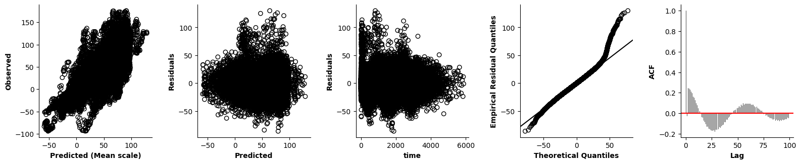
The model’s still not perfect - but the acf plot, the predicted vs. residuals plot, and the time vs. residuals plot are all far less concerning (note how the “stringing” in the last two disappeared almost completely). To improve the model further, we might want to include random intercepts per series. Additionally, we could try different values for rho. We could even select rho formally - by picking the model with the highest reml score (e.g., Wood et al., 2015). If you want to set up such a grid-search over different values of rho, the reml score is available via model.get_reml().
ar1 Model for Generalized Models
Like the bam function in mgcv, the GAMM class in mssm also allows to include an “ar1” model for generalized (and also extended) models - the “ar1” model is then applied to the “working residuals” of the linearized model (see Wood, 2017). Below we show an example for a Gamma model:
# We simulate some data including a random smooth - but then dont include it in the model:
sim_dat = sim11(5000,2,c=0,seed=20,family=Gamma(),n_ranef=20,binom_offset = 0)

sim_dat = sim_dat.sort_values(['x4'], ascending=[True])

sim_formula = Formula(lhs("y"),
                      [i(),f(["x0"]),f(["x1"]),f(["x2"]),f(["x3"])],
                      data=sim_dat,
                      series_id="x4") # Can already specify this.

gamma_model2 = GAMM(sim_formula,Gamma())
gamma_model2.fit(progress_bar=False)
Both the plot of the deviance residuals and the plot of the pearson residuals shows some auto-correlation. Let’s try and improve this by including an “ar1” model:
fig = plt.figure(figsize=(5*single_size,single_size),layout='constrained')
axs = fig.subplots(1,5,gridspec_kw={"wspace":0.1})
plot_val(gamma_model2,pred_viz=["x0"],resid_type="Pearson",axs=axs)
axs[-1].set_ylim([-0.2,1])
(-0.2, 1.0)
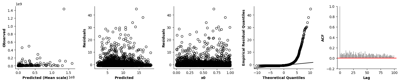
gamma_model2.fit(rho=0.25,restart=True,progress_bar=False)
The model slightly improves when including an “ar1” model:
fig = plt.figure(figsize=(5*single_size,single_size),layout='constrained')
axs = fig.subplots(1,5,gridspec_kw={"wspace":0.1})
plot_val(gamma_model2,pred_viz=["x0"],resid_type="ar1",axs=axs)
axs[-1].set_ylim([-0.2,1])
(-0.2, 1.0)
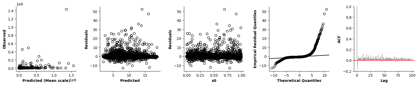
We could try and include random intercepts per level of “x4” to further improve the model.
Posterior Simulation & Whole-interval CIs
In the section on model selection we briefly dicussed CIs, and pointed out that they offer an additional tool to check whether a function should be included in the model or not. Importantly, the CIs visualized so far are point-wise CIs, but to determine whether a function should be included in the model at all, whole-function CIs are more appropriate. Point-wise CIs include the true function on average at 95% of the values evaluated - but that rate might be higher or lower for some combination of predictor values over which the interval is evaluated (i.e., the coverage is truly achieved “on average”; see Wood, 2017). Whole-function CIs on the other hand are modified to encapsulate the true function at every evaluated predictor combination with a certain probability (see Wood, 2017 but also Simpson, 2016 for more details) - i.e., they ensure that the entire true function falls within the CI boundaries with 95% certainty.
The difference can be visualized best by simulating from the conditional posterior distribution of a GAM(M). Wood (2017) shows that the latter is approximately \(\beta | \lambda,y \sim N(\hat{\beta},\mathbf{V})\). Where \(\mathbf{V}\) is the inverse of the ngeative Hessian of the penalized likelihood. By defining model-matrix \(\hat{\mathbf{X}}\) to only contain non-zero entries in the columns related to some function of interest \(f\), we can use this result to simulate replications of \(f\).
Below we sample from the posterior of f["time"] for level “a” of factor “cond” from model 10:
# Set up some new data for prediction
tr = np.linspace(0,4000,30)

pred_dat = pd.DataFrame({"time":tr,
                        "x":[-1 for _ in range(len(tr))],
                        "cond":["a" for _ in range(len(tr))],
                        "series":[0 for _ in range(len(tr))]})

_,pred_mat,_ = model10.predict([2],pred_dat)
# `use_post` identifies only coefficients related to f(time) - and only for condition a
use_post = pred_mat.sum(axis=0) != 0
use_post = np.arange(0,pred_mat.shape[1])[use_post]
use_post
array([ 2, 3, 4, 5, 6, 7, 8, 9, 10])
# Now we can sample new realizations of f(time) from the conditional posterior
# By default all plotting functions will draw 10.000 samples from the posterior so we specify this for the manual sampling below.
post = model10.sample_post(10000,use_post,seed=2000)
post_f = pred_mat[:,use_post] @ post
# And plot the replications against a point-wise and a whole-function CI
fig = plt.figure(figsize=(2*single_size,single_size),layout='constrained')
axs = fig.subplots(1,2,gridspec_kw={"wspace":0.1})

for sim in range(100):
    axs[0].plot(pred_dat["time"],post_f[:,sim],alpha=0.3)

plot_fitted(pred_dat,["time"],model10,[2],ax=axs[0],plot_exist=False,col=0.1)

for sim in range(100):
    axs[1].plot(pred_dat["time"],post_f[:,sim],alpha=0.3)

# This time, we set the whole-interval argument to `True`.
plot_fitted(pred_dat,["time"],model10,[2],ax=axs[1],whole_interval=True,plot_exist=False,col=0.1)

plt.show()
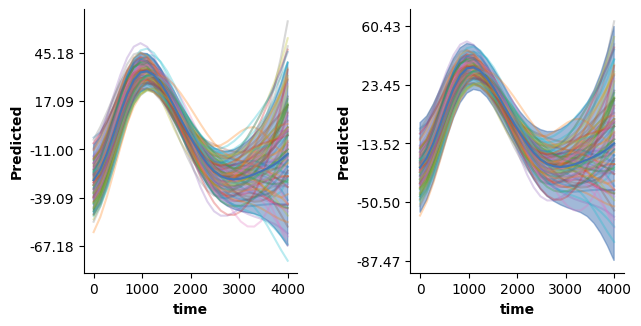
Evidently, while the point-wise CI covers the simulated replications consistently over some time values, there are quite a few curves that do not fall within the CI boundaries when considering the entire time range. For the whole-function CI most replicate functions are completely encapsulated.
To clarify, the point-wise CI is not performing poorly here! In fact, the check below confirms that - on average over time - it contains simulated replicates in 95% across simulations. However, only in around 75% of simulations does it contain the function over the whole time range - but it was simply not designed to achieve this!
# Get the boundaries shown in the left plot and check them against each replicate function
# drawn from the posterior.
pred,pred_mat,b = model10.predict([2],pred_dat,whole_interval=False,seed=2000,ci=True)

avg = []
full_cov = 0
for pi in range(post_f.shape[1]):
    IN_CI = ((pred + b) > post_f[:,pi]) & ((pred - b) < post_f[:,pi])
    if not False in np.unique(IN_CI):
        full_cov += 1

    avg.append(len(pred[IN_CI])/len(pred))

full_cov/=post_f.shape[1]
print(np.mean(avg))
print(full_cov)
0.95057
0.7417
We can now run the same check for the whole-function CI. Note that for the check a different seed is used (otherwise coverage would be exactly 95%). Nevertheless, the whole-function CI covers the entire replicate in approximately 95% of simulations. In terms of average coverage it over-performs (naturally) - achieving a point-wise coverage of almost 99%. This is only logical, considering that the interval is simply expanded - relative to the point-wise CI (see Wood et al., 2016).
# Get the boundaries shown in the right plot and check them against each replicate function
# drawn from the posterior.
pred,pred_mat,b = model10.predict([2],pred_dat,whole_interval=True,seed=1500,ci=True)

avg = []
full_cov = 0
for pi in range(post_f.shape[1]):
    IN_CI = ((pred + b) > post_f[:,pi]) & ((pred - b) < post_f[:,pi])
    if not False in np.unique(IN_CI):
        full_cov += 1

    avg.append(len(pred[IN_CI])/len(pred))

full_cov/=post_f.shape[1]
print(np.mean(avg))
print(full_cov)
0.9933
0.9533
This quick comparison highlights, that if you want to check whether a smooth has any effect, i.e., whether it should be included in the model, whole-function CIs are much more appropriate, simply because they test this more explicitly. That is: if the whole-function CI for a smooth contains zero at every evaluated predictor combination, it is probably safe to assume that the effect can be dropped from the model.
Posterior Simulation & Whole-interval CIs for GAMMLSS and GSMM models
The api to sample from the posterior of a GAMMLSS or GSMM model is very similar - the only difference is that model.sample_post works for a specified parameter of the log-likelihood/response variables. This is illustrated below. We consider the complex GAMMLSS example we introduced above:
gaumlss_model2.print_smooth_terms()
Distribution parameter: 1

f(['x0']); edf: 4.146
f(['x1']); edf: 5.709
f(['x0'],by=x4); edf: 110.674

Distribution parameter: 2

f(['x2']); edf: 7.339
f(['x3']); edf: 1.001
In this model, two parameters of the log-likelihood (the mean and scale parameter) were specified as additive models - both of which involve smooth functions. Now let’s say we want to sample the posterior of f(["x0"]) included in the model of the mean. To achieve this, we largely proceed as we did for the GAMM model. We start with setting up new data.
# Set up some new data for prediction
pred_dat = pd.DataFrame({"x0":np.linspace(0,1,30),
                         "x1":np.linspace(0,1,30),
                         "x4":[gaumlss_model2.formulas[0].coding_factors["x4"][0] for _ in range(30)]})

_,pred_mat,_ = gaumlss_model2.predict([1],pred_dat,par=0)
Note, that we only had to include values in pred_dat for variables associated with the first formula. Now we can again figure out for which coefficients we want to sample the posterior:
# `use_post` identifies only coefficients related to f(x0)
use_post = pred_mat.sum(axis=0) != 0
use_post = np.arange(0,pred_mat.shape[1])[use_post]
use_post
array([1, 2, 3, 4, 5, 6, 7, 8, 9])
Now we are ready to sample the posterior:
# Now we can sample new realizations of f(x0) from the conditional posterior
# By default all plotting functions will draw 10.000 samples from the posterior so we specify this for the manual sampling below.
post = gaumlss_model2.sample_post(10000,use_post,seed=2000)
post_f = pred_mat[:,use_post] @ post
# And plot the replications against a point-wise and a whole-function CI
fig = plt.figure(figsize=(2*single_size,single_size),layout='constrained')
axs = fig.subplots(1,2,gridspec_kw={"wspace":0.1})

for sim in range(100):
    axs[0].plot(pred_dat["x1"],post_f[:,sim],alpha=0.3)

plot(gaumlss_model2,which=[1],axs=[axs[0]],prov_cols=0.1)

for sim in range(100):
    axs[1].plot(pred_dat["x1"],post_f[:,sim],alpha=0.3)

# This time, we set the whole-interval argument to `True`.
plot(gaumlss_model2,which=[1],axs=[axs[1]],whole_interval=True,prov_cols=0.1)

plt.show()
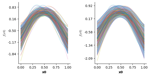
All in all, this was not that different from sampling the posterior for a GAMM, right? Right! Now, let’s look at sampling the posterior of f["x2"] in the model of the scale paramter. The steps are the same, the important thing is that we set par=1 when calling gaumlss_model2.predict. We still set use_terms=[1] since we want the second term (first smooth term) in the formula/model of the scale parameter:
# Set up some new data for prediction - this time for scale parameter
pred_dat = pd.DataFrame({"x2":np.linspace(0,1,30),
                         "x3":np.linspace(0,1,30)})

_,pred_mat,_ = gaumlss_model2.predict([1],pred_dat,par=1)
# `use_post` identifies only coefficients related to f(x2) in the model of the scale parameter
use_post = pred_mat.sum(axis=0) != 0
use_post = np.arange(0,pred_mat.shape[1])[use_post]
use_post
array([1, 2, 3, 4, 5, 6, 7, 8, 9])
Now, the step to figure out which coefficients we need might be a bit confusing - after all the indices are the same we got when sampling from the model of the mean. However, this is intended - as clarified by looking what it says under use_post in the doc string of the .sample_post function:
help(gaumlss_model.sample_post)
Help on method sample_post in module mssm.models:

sample_post(
    n_ps: int,
    use_post: list[int] | None = None,
    deviations: bool = False,
    seed: int | None = None,
    par: int = 0
) -> np.ndarray method of mssm.models.GAMMLSS instance
    Obtain ``n_ps`` samples from posterior :math:`[\boldsymbol{\beta}_m -         \hat{\boldsymbol{\beta}}_m] | \mathbf{y},\boldsymbol{\lambda} \sim N(0,\mathbf{V})`,
    where :math:`\mathbf{V}=[-\mathbf{H} + \mathbf{S}_{\lambda}]^{-1}`
    (see Wood et al., 2016; Wood 2017, section 6.10), :math:`\boldsymbol{\beta}_m` is
    the set of coefficients in the model of parameter :math:`m` of the distribution
    (see argument ``par``), and :math:`\mathbf{H}` is the hessian of the log-likelihood
    (Wood et al., 2016;). To obtain samples for :math:`\boldsymbol{\beta}`, set ``deviations``
    to false.

    see :func:`sample_MVN` for more details.

    Examples::

        from mssm.models import *
        from mssmViz.sim import *
        from mssmViz.plot import *
        import matplotlib.pyplot as plt

        # Simulate 500 data points
        GAUMLSSDat = sim6(500,seed=20)

        # We need to model the mean: \mu_i = \alpha + f(x0)
        formula_m = Formula(lhs("y"),
                            [i(),f(["x0"],nk=10)],
                            data=GAUMLSSDat)

        # and the standard deviation as well: log(\sigma_i) = \alpha + f(x0)
        formula_sd = Formula(lhs("y"),
                            [i(),f(["x0"],nk=10)],
                            data=GAUMLSSDat)

        # Collect both formulas
        formulas = [formula_m,formula_sd]

        # Create Gaussian GAMMLSS family with identity link for mean
        # and log link for sigma
        family = GAUMLSS([Identity(),LOG()])

        # Now fit
        model = GAMMLSS(formulas,family)
        model.fit()

        new_dat = pd.DataFrame({"x0":np.linspace(0,1,30)})

        # Now obtain the estimate for `f(["x0"],nk=10)` and the model matrix corresponding to
        # it! Note, that we set `use_terms = [1]` - so all columns in X_f not belonging to
        # `f(["x0"],nk=10)` (e.g., the first one, belonging to the offset) are zeroed.
        mu_f,X_f,_ = model.predict([1],new_dat,ci=True)

        # Now we can sample from the posterior of `f(["x0"],nk=10)` in the model of the mean:
        post = model.sample_post(10000,None,deviations=False,seed=0,par=0)

        # Since we set deviations to false post has coefficient samples and can simply be
        # post-multiplied to get samples of `f(["x0"],nk=10)`
        post_f = X_f @ post

        # Plot the estimated effect and 50 posterior samples
        plt.plot(new_dat["x0"],mu_f,color="black",linewidth=2)

        for sidx in range(50):
            plt.plot(new_dat["x0"],post_f[:,sidx],alpha=0.2)

        plt.show()

        # In this case, we are not interested in the offset, so we can omit it during the
        # sampling step (i.e., to not sample coefficients for it):

        # `use_post` identifies only coefficients related to `f(["x0"],nk=10)`
        use_post = X_f.sum(axis=0) != 0
        use_post = np.arange(0,X_f.shape[1])[use_post]
        print(use_post)

        # `use_post` can now be passed to `sample_post`:
        post2 = model.sample_post(10000,use_post,deviations=False,seed=0,par=0)

        # Importantly, post2 now has a different shape - which we have to take into account
        # when multiplying.
        post_f2 = X_f[:,use_post] @ post2

        plt.plot(new_dat["x0"],mu_f,color="black",linewidth=2)

        for sidx in range(50):
            plt.plot(new_dat["x0"],post_f2[:,sidx],alpha=0.2)

        plt.show()

    References:
     - Wood, Pya, & Säfken (2016). Smoothing Parameter and Model Selection for General             Smooth Models.
     - Wood, S. N. (2017). Generalized Additive Models: An Introduction with R, Second             Edition (2nd ed.).

    :param n_ps: Number of samples to obtain from posterior.
    :type n_ps: int,optional
    :param use_post: The indices corresponding to coefficients for which to actually obtain
        samples. **Note**: an index of 0 indexes the first coefficient in the model of
        parameter ``par``, that is indices have to correspond to columns in the
        parameter-specific model matrix. By default all coefficients are sampled.
    :type use_post: [int],optional
    :param deviations: Whether to return samples of **deviations** from the estimated
        coefficients (i.e., :math:`\boldsymbol{\beta} - \hat{\boldsymbol{\beta}}`)
        or actual samples of coefficients (i.e., :math:`\boldsymbol{\beta}`), defaults to
        False
    :type deviations: bool,optional
    :param seed: A seed to use for the sampling, defaults to None
    :type seed: int,optional
    :param par: The index corresponding to the distribution parameter for which to make the
        prediction (e.g., 0 = mean)
    :type par: int
    :returns: An np.ndarray of dimension ``[len(use_post),n_ps]`` containing the posterior
        samples. Can simply be post-multiplied with model matrix :math:`\mathbf{X}` to
        generate posterior **sample curves**.
    :rtype: np.ndarray
So .sample_post expects indices with respect to the number of coefficients in the chosen formula/model (i.e., indicated via par). Now, the second formula starts with an intercept term, just like the first one. Hence, the first coefficient associated with f(["x2"]) in the model of the scale parameter makes up the second column of the model matrix - corresponding to index 1. Thus, the returned indices are correct and we can proceed with sampling the posterior. Importantly, we again have to specify the par parameter and set it to 1:
Note: if you set the same seed when sampling the posterior for different parameters, exactly the same coefficient samples will be generated for all individual parameters - so it will be like sampling the posterior of all parameters simultaneously.
# Now we can sample new realizations of f(x2) from the conditional posterior
post = gaumlss_model2.sample_post(10000,use_post,seed=2000,par=1)
post_f = pred_mat[:,use_post] @ post
Finally, we can plot - again taking care to specify dist_par=1 wherever needed:
# And plot the replications against a point-wise and a whole-function CI
fig = plt.figure(figsize=(2*single_size,single_size),layout='constrained')
axs = fig.subplots(1,2,gridspec_kw={"wspace":0.1})

for sim in range(100):
    axs[0].plot(pred_dat["x2"],post_f[:,sim],alpha=0.3)

plot(gaumlss_model2,which=[1],axs=[axs[0]],prov_cols=0.1,dist_par=1)

for sim in range(100):
    axs[1].plot(pred_dat["x2"],post_f[:,sim],alpha=0.3)

# This time, we set the whole-interval argument to `True`.
plot(gaumlss_model2,which=[1],axs=[axs[1]],whole_interval=True,prov_cols=0.1,dist_par=1)

plt.show()
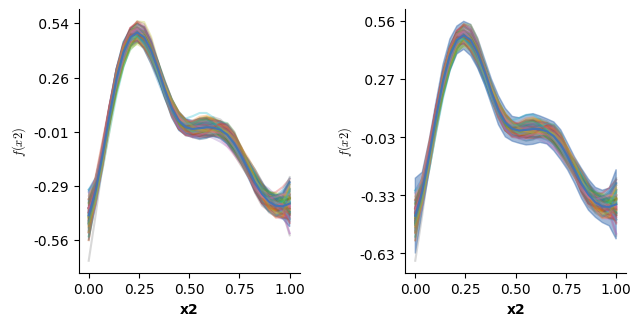
Fully Bayesian Inference & exact (Bayesian) Posterior Simulation
The previous section showed how to sample from the normal approximation to the conditional posterior of the model coefficients given an estimate of the smoothing penalties/regularization parameters \(\beta | \lambda,y \sim N(\hat{\beta},\mathbf{V})\). The normal approximation is easily justified for models of a lot of data involving a moderate number of coefficients (see Wood et al., 2016 for details), but can occasionally produce poor results (especially for binary data). Therefore, we may ocassionally want to perform fully Bayesian inference about the exact (Bayesian) posterior. Another reason for this, is that doing so allows us to consider the joint posterior \(p(\beta,\rho, \theta | y)\) of the model coefficients \(\beta\), log smoothing penalties \(\rho = log(\lambda)\), and additional parameters of the model’s likelihood \(\theta\) like \(\phi\) (the scale parameter of GAMMs) given data \(y\).
Fully Bayesian inference requires that priors are placed on \(\rho\), \(\theta\), and any coefficients left-unpenalized in conventional smooth models (this includes the space of smooth functions left un-penalized by the default penalties, for a detailed discussion see Wood, 2016). Technically, this is not absolutely necessary, since we can leave the prior improper, but mssm anyways selects very vagues priors for these parameters by default - which are unlikely to strongly affect the sampled parameters but can nevertheless improve the stability of the sampling. However, if you really want an improper prior, mssm supports that as well (just like it allows you to choose stronger/more informative priors for the aforementioned parameters).
To sample from the Bayesian posterior, we first need to import the sample_mssm function:
from mssm.src.python.mcmc import sample_mssm
Below we tell the function to sample the conditional (still exact) posterior \(p(\beta | y, \rho)\) of model gaumlss_model2. In this example we sample the conditional rather than the joint posterior \(p(\beta,\rho | y)\) (sample_rho=False, the default), since sampling the joint will take much longer. We also specified a short adaptation period (M_adapt=20) and obtain only a small number of samples n_iter=1000. In practice, the default values are far more reasonable. Note, that sample_mssm by default automatically decides on an appropriate effective sample size and whether the chain is sufficiently converged (auto_converge=True, note that in practice you should always inspect the samples to make sure that the chain has indeed converged sufficiently and produced an acceptable effective sample size). Thus, just because n_iter=10000 by default, it does not mean that the sampler will run for this long. By default sample_mssm obtains samples from two chains in parallel (n_chains=2 and parallelize_chains=True). We do not reccomend sampling only a single chain - instead, in practice you will probably want to sample from at least 4-8 chains in parallel (this also improves the usefulness of the auto_converge feature).
# Obtain samples from the conditional posterior
chains = sample_mssm(gaumlss_model2,M_adapt=20,n_iter=1000,sample_rho=False,progress_bar=False)
We can now re-create the plot illustrating the whole-interval CIs from the previous section, but instead of plotting curves from the normal approximation to the conditional posterior we plot curves from the Bayesian conditional posterior. Before we can do this, we will need to extract the coefficients associated with the standard deviation parameter from the chains object. Specifically, while the sample_post method accepted an argument to sample only the coefficients associated with the second parameter of the log-likelihood (i.e., par=1 - here corresponding to the standard deviation), the chains object holds all coefficients:
chains.coefs.shape
(2, 1000, 228)
The first dimension corresponds to the number of chains sampled, the second to the number of samples obtained, and the third matches the total coefficients required by the model:
gaumlss_model2.coef.shape
(228, 1)
We can use np.split together with the gaumlss_model2.coef_split_idx object to split the coefficients into separate sets per likelihood parameter:
split_post_coef = np.split(chains.coefs,gaumlss_model2.coef_split_idx,axis=2)

print(split_post_coef[0].shape,split_post_coef[1].shape)
(2, 1000, 209) (2, 1000, 19)
Now, split_post_coef[1] holds only coefficients associated with par=1, and we can use these as before to produce sampled curves - below we do this separately for the two chains:
post_f1 = pred_mat[:,use_post] @ split_post_coef[1][0,:,use_post]
post_f2 = pred_mat[:,use_post] @ split_post_coef[1][1,:,use_post]
Now we can replicate the plot from the previous section - this time we plot 50 curves per chain from the Bayesian posterior. Note, that the curves from the Bayesian posterior are less smooth and also exceed the whole-interval CI more often than expected. If we had sampled the joint posterior, you could expect even more variation!
# Plot the Bayesian posterior curve samples against a point-wise and a whole-function CI
fig = plt.figure(figsize=(2*single_size,single_size),layout='constrained')
axs = fig.subplots(1,2,gridspec_kw={"wspace":0.1})

for sim in range(100):
    if sim < 50:
        axs[0].plot(pred_dat["x2"],post_f1[:,sim],alpha=0.3)
    else:
        axs[0].plot(pred_dat["x2"],post_f2[:,sim],alpha=0.3)

plot(gaumlss_model2,which=[1],axs=[axs[0]],prov_cols=0.1,dist_par=1)

for sim in range(100):
    if sim < 50:
        axs[1].plot(pred_dat["x2"],post_f1[:,sim],alpha=0.3)
    else:
        axs[1].plot(pred_dat["x2"],post_f2[:,sim],alpha=0.3)

# Again, we set the whole-interval argument to `True`.
plot(gaumlss_model2,which=[1],axs=[axs[1]],whole_interval=True,prov_cols=0.1,dist_par=1)

plt.show()
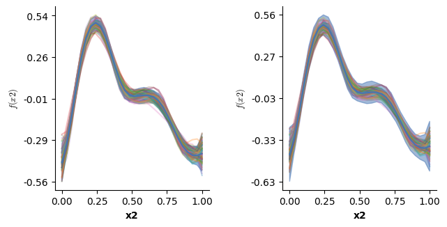
The GSMM Class in mssm
The GSMM class supports the most generic smooth models, as defined by Wood, Pya, and Säfken (2016; see also Krause et al., submitted). Essentially, it allows to estimate any model with a regular likelihood - the parameters of which can be specified as smooth models. An intriguing aspect of the GSMM class, is that it can rely on the L-qEFS algorithm (Krause et al., submitted) to estimate these models. When relying on the L-qEFS algorithm, mssm only requires researchers to code up the log-likelihood of the model they want to estimate. In this section we show how this could look like. We work with a simple example - and just imagine for now that we completely forgot how to estimate a Gaussian model of location, scale and shape.
The first thing we need to do to estimate a GSMM is to implement the GSMMFamily class. We can again look at the help function to get an idea of what that entails:
help(GSMMFamily)
Help on class GSMMFamily in module mssm.src.python.exp_fam:

class GSMMFamily(builtins.object)
 |  GSMMFamily(pars: int, links: list[Link], *llkargs) -> None
 |
 |  Base-class for General Smooth "families" as discussed by Wood, Pya, & Säfken (2016).
 |  For estimation of :class:`mssm.models.GSMM` models via ``L-qEFS`` (Krause et al., submitted) it
 |  is sufficient to implement :func:`llk`. :func:`gradient` and :func:`hessian` can then simply
 |  return ``None``. For exact estimation via Newton's method, the latter two functions need to be
 |  implemented and have to return the gradient and hessian at the current coefficient estimate
 |  respectively.
 |
 |  Additional parameters needed for likelihood, gradient, or hessian evaluation can be passed
 |  along via the ``llkargs``. They are then made available in ``self.llkargs``.
 |
 |  References:
 |   - Wood, Pya, & Säfken (2016). Smoothing Parameter and Model Selection for General         Smooth Models.
 |   - Nocedal & Wright (2006). Numerical Optimization. Springer New York.
 |   - Krause et al. (submitted). The Mixed-Sparse-Smooth-Model Toolbox (MSSM): Efficient         Estimation and Selection of Large Multi-Level Statistical Models.         https://doi.org/10.48550/arXiv.2506.13132
 |
 |  :param pars: Number of parameters of the likelihood for which an additive (mixed) model is
 |      specified. **Note**, that extra parameters that are constant (and thus do not need an
 |      extra :class:`mssm.src.python.formula.Formula` specified) but nevertheless need to be
 |      estimated can be handled via the ``extra_coef`` argument.
 |  :type pars: int
 |  :param links: List of Link functions for each parameter of the likelihood,
 |      e.g., `links=[Identity(),LOG()]`.
 |  :type links: [Link]
 |  :ivar int, optional extra_coef: Number of extra coefficients required by specific family for
 |      parameters of the log-likelihood that are constant (i.e., not a function of predictor
 |      variables) or ``None``. If this is not set to ``None``, ``mssm`` will automatically append
 |      ``extra_coef`` elements to the coefficient vector passed to the log-likelihood and gradient
 |      methods of this family. Additionally, ``coef_split_idx`` will be modified, so that the last
 |      list of the split holds the ``extra_coef``. By default set to ``None`` and changed to
 |      ``int`` by specific families requiring this.
 |  :ivar list[any] llkargs: A list holding any extra arguments passed to the constructor via
 |      ``llkargs``.
 |
 |  Methods defined here:
 |
 |  __init__(self, pars: int, links: list[Link], *llkargs) -> None
 |      Initialize self.  See help(type(self)) for accurate signature.
 |
 |  get_resid(
 |      self,
 |      coef: np.ndarray,
 |      coef_split_idx: list[int],
 |      ys: list[np.ndarray | None],
 |      Xs: list[scp.sparse.csc_array | None],
 |      **kwargs
 |  ) -> np.ndarray | None
 |      Get standardized residuals for a GSMM model.
 |
 |      Any implementation of this function should return a vector that looks like what could be
 |      expected from taking independent draws from :math:`N(0,1)`. Any additional arguments
 |      required by a specific implementation can be passed along via ``kwargs``.
 |
 |      **Note**: Families for which no residuals are available can return None.
 |
 |      References:
 |       - Wood, Pya, & Säfken (2016). Smoothing Parameter and Model Selection for General             Smooth Models.
 |       - Wood, S. N. (2017). Generalized Additive Models: An Introduction with R, Second             Edition (2nd ed.).
 |
 |      :param coef: The current coefficient estimate (as np.array of shape (-1,1) - so it must
 |          not be flattened!).
 |      :type coef: np.ndarray
 |      :param coef_split_idx: A list used to split (via :func:`np.split`) the ``coef`` into the
 |          sub-sets associated with each paramter of the llk.
 |      :type coef_split_idx: [int]
 |      :param ys: List containing the vectors of observations (each of shape (-1,1)) passed as
 |          ``lhs.variable`` to the formulas. **Note**: by convention ``mssm`` expectes that the
 |          actual observed data is passed along via the first formula (so it is stored in
 |          ``ys[0]``). If multiple formulas have the same ``lhs.variable`` as this first formula,
 |          then ``ys`` contains ``None`` at their indices to save memory.
 |      :type ys: list[np.ndarray | None]
 |      :param Xs: A list of sparse model matrices per likelihood parameter. Might contain ``None``
 |          at indices for matrices which were flagged as "do not build" via the ``build_mat``
 |          argument of the :func:`mssm.models.GSMM.fit` method.
 |      :type Xs: list[scp.sparse.csc_array | None]
 |      :return: a vector of shape (-1,1) containing standardized residuals under the current model
 |          (**Note**, the first axis will not necessarily match the dimension of any of the
 |          response vectors (this will depend on the specific Family's implementation)) or None in
 |          case residuals are not readily available.
 |      :rtype: np.ndarray | None
 |
 |  gradient(
 |      self,
 |      coef: np.ndarray,
 |      coef_split_idx: list[int],
 |      ys: list[np.ndarray | None],
 |      Xs: list[scp.sparse.csc_array | None]
 |  ) -> np.ndarray
 |      Function to evaluate the gradient of the llk at current coefficient estimate ``coef``.
 |
 |      By default relies on numerical differentiation as implemented in scipy to approximate the
 |      Gradient from the implemented log-likelihood function. See the link in the references for
 |      more details.
 |
 |      References:
 |         - Wood, Pya, & Säfken (2016). Smoothing Parameter and Model Selection for General             Smooth Models.
 |         - ``scipy.optimize.approx_fprime``: at             https://docs.scipy.org/doc/scipy/reference/generated/scipy.optimize.approx_fprime.html
 |         - Krause et al. (submitted). The Mixed-Sparse-Smooth-Model Toolbox (MSSM): Efficient             Estimation and Selection of Large Multi-Level Statistical Models.             https://doi.org/10.48550/arXiv.2506.13132
 |
 |      :param coef: The current coefficient estimate (as np.array of shape (-1,1) - so it must not
 |          be flattened!).
 |      :type coef: np.ndarray
 |      :param coef_split_idx: A list used to split (via :func:`np.split`) the ``coef`` into the
 |          sub-sets associated with each paramter of the llk.
 |      :type coef_split_idx: [int]
 |      :param ys: List containing the vectors of observations (each of shape (-1,1)) passed as
 |          ``lhs.variable`` to the formulas. **Note**: by convention ``mssm`` expectes that the
 |          actual observed data is passed along via the first formula (so it is stored in
 |          ``ys[0]``). If multiple formulas have the same ``lhs.variable`` as this first formula,
 |          then ``ys`` contains ``None`` at their indices to save memory.
 |      :type ys: list[np.ndarray | None]
 |      :param Xs: A list of sparse model matrices per likelihood parameter. Might contain ``None``
 |          at indices for matrices which were flagged as "do not build" via the ``build_mat``
 |          argument of the :func:`mssm.models.GSMM.fit` method.
 |      :type Xs: list[scp.sparse.csc_array | None]
 |      :return: The Gradient of the log-likelihood evaluated at ``coef`` as numpy array of
 |          shape (-1,1).
 |      :rtype: np.ndarray
 |
 |  hessian(
 |      self,
 |      coef: np.ndarray,
 |      coef_split_idx: list[int],
 |      ys: list[np.ndarray | None],
 |      Xs: list[scp.sparse.csc_array | None]
 |  ) -> scp.sparse.csc_array
 |      Function to evaluate the hessian of the llk at current coefficient estimate ``coef``.
 |
 |      Only has to be implemented if full Newton is to be used to estimate coefficients. If the
 |      L-qEFS update by Krause et al. (in preparation) is to be used instead, this method does not
 |      have to be implemented.
 |
 |      References:
 |         - Wood, Pya, & Säfken (2016). Smoothing Parameter and Model Selection for General             Smooth Models.
 |         - ``scipy.optimize.approx_fprime``: at             https://docs.scipy.org/doc/scipy/reference/generated/scipy.optimize.approx_fprime.html
 |         - Krause et al. (submitted). The Mixed-Sparse-Smooth-Model Toolbox (MSSM): Efficient             Estimation and Selection of Large Multi-Level Statistical Models.             https://doi.org/10.48550/arXiv.2506.13132
 |
 |      :param coef: The current coefficient estimate (as np.array of shape (-1,1) - so it must not
 |          be flattened!).
 |      :type coef: np.ndarray
 |      :param coef_split_idx: A list used to split (via :func:`np.split`) the ``coef`` into the
 |          sub-sets associated with each paramter of the llk.
 |      :type coef_split_idx: [int]
 |      :param ys: List containing the vectors of observations (each of shape (-1,1)) passed as
 |          ``lhs.variable`` to the formulas. **Note**: by convention ``mssm`` expectes that the
 |          actual observed data is passed along via the first formula (so it is stored in
 |          ``ys[0]``). If multiple formulas have the same ``lhs.variable`` as this first formula,
 |          then ``ys`` contains ``None`` at their indices to save memory.
 |      :type ys: list[np.ndarray | None]
 |      :param Xs: A list of sparse model matrices per likelihood parameter. Might contain ``None``
 |          at indices for matrices which were flagged as "do not build" via the ``build_mat``
 |          argument of the :func:`mssm.models.GSMM.fit` method.
 |      :type Xs: list[scp.sparse.csc_array | None]
 |      :return: The Hessian of the log-likelihood evaluated at ``coef``.
 |      :rtype: scp.sparse.csc_array
 |
 |  init_coef(self, models: list[Callable]) -> np.ndarray
 |      (Optional) Function to initialize the coefficients of the model.
 |
 |      Can return ``None`` , in which case random initialization will be used.
 |
 |      :param models: A list of :class:`mssm.models.GAMM`'s, - each based on one of the formulas
 |          provided to a model.
 |      :type models: [mssm.models.GAMM]
 |      :return: A numpy array of shape (-1,1), holding initial values for all model coefficients.
 |      :rtype: np.ndarray
 |
 |  init_lambda(self, penalties: list[Callable]) -> list[float]
 |      (Optional) Function to initialize the smoothing parameters of the model.
 |
 |      Can return ``None`` , in which case random initialization will be used.
 |
 |      :param penalties: A list of all penalties to be estimated by the model.
 |      :type penalties: [mssm.src.python.penalties.LambdaTerm]
 |      :return: A list, holding - for each :math:`\lambda` parameter to be estimated - an initial
 |          value.
 |      :rtype: np.ndarray
 |
 |  jhessian(
 |      self,
 |      jcols: np.ndarray,
 |      coef: np.ndarray,
 |      coef_split_idx: list[int],
 |      ys: list[np.ndarray | None],
 |      Xs: list[scp.sparse.csc_array | None],
 |      n_c: int = 1
 |  ) -> scp.sparse.csc_array
 |      (Optional) method to compute a sparse approximation to the Hessian of the llk, containing
 |      only the ``j`` columns and rows of the Hessian indexed by ``jcols``.
 |
 |      By default the method relies on a finite difference approximation to evaluate the ``j``
 |      columns of the Hessian of the llk. Result is returned as symmetric sparse matrix.
 |
 |      :param jcols: Array holding indices of columns to approximate.
 |      :type jcols: np.ndarray
 |      :param coef: The current coefficient estimate (as np.array of shape (-1,1) - so it must not
 |          be flattened!).
 |      :type coef: np.ndarray
 |      :param coef_split_idx: A list used to split (via :func:`np.split`) the ``coef`` into the
 |          sub-sets associated with each paramter of the llk.
 |      :type coef_split_idx: [int]
 |      :param ys: List containing the vectors of observations (each of shape (-1,1)) passed as
 |          ``lhs.variable`` to the formulas. **Note**: by convention ``mssm`` expectes that the
 |          actual observed data is passed along via the first formula (so it is stored in
 |          ``ys[0]``). If multiple formulas have the same ``lhs.variable`` as this first formula,
 |          then ``ys`` contains ``None`` at their indices to save memory.
 |      :type ys: list[np.ndarray | None]
 |      :param Xs: A list of sparse model matrices per likelihood parameter. Might contain ``None``
 |          at indices for matrices which were flagged as "do not build" via the ``build_mat``
 |          argument of the :func:`mssm.models.GSMM.fit` method.
 |      :type Xs: list[scp.sparse.csc_array | None]
 |      :param n_c: Number of cores to use to parallelize computation over ``j`` cols, defaults to
 |          1.
 |      :type n_c: int, optional
 |      :return: Finite difference approximation matrix which is symmetric sparse matrix with
 |          ``jcols`` rows and columns set to finite difference approximation of columns of
 |          Hessian of llk
 |      :rtype: scp.sparse.csc_array
 |
 |  llk(
 |      self,
 |      coef: np.ndarray,
 |      coef_split_idx: list[int],
 |      ys: list[np.ndarray | None],
 |      Xs: list[scp.sparse.csc_array | None]
 |  ) -> float
 |      log-probability of data under given model.
 |
 |      References:
 |       - Wood, Pya, & Säfken (2016). Smoothing Parameter and Model Selection for General             Smooth Models.
 |       - Wood, S. N. (2017). Generalized Additive Models: An Introduction with R, Second             Edition (2nd ed.).
 |       - Krause et al. (submitted). The Mixed-Sparse-Smooth-Model Toolbox (MSSM): Efficient             Estimation and Selection of Large Multi-Level Statistical Models.             https://doi.org/10.48550/arXiv.2506.13132
 |
 |      :param coef: The current coefficient estimate (as np.array of shape (-1,1) - so it must not
 |          be flattened!).
 |      :type coef: np.ndarray
 |      :param coef_split_idx: A list used to split (via :func:`np.split`) the ``coef`` into the
 |          sub-sets associated with each paramter of the llk.
 |      :type coef_split_idx: [int]
 |      :param ys: List containing the vectors of observations (each of shape (-1,1)) passed as
 |          ``lhs.variable`` to the formulas. **Note**: by convention ``mssm`` expectes that the
 |          actual observed data is passed along via the first formula (so it is stored in
 |          ``ys[0]``). If multiple formulas have the same ``lhs.variable`` as this first formula,
 |          then ``ys`` contains ``None`` at their indices to save memory.
 |      :type ys: list[np.ndarray | None]
 |      :param Xs: A list of sparse model matrices per likelihood parameter. Might contain ``None``
 |          at indices for matrices which were flagged as "do not build" via the ``build_mat``
 |          argument of the :func:`mssm.models.GSMM.fit` method.
 |      :type Xs: list[scp.sparse.csc_array | None]
 |      :return: The log-likelihood evaluated at ``coef``.
 |      :rtype: float
 |
 |  ----------------------------------------------------------------------
 |  Data descriptors defined here:
 |
 |  __dict__
 |      dictionary for instance variables
 |
 |  __weakref__
 |      list of weak references to the object
As mentioned, this again states that we only need to implement the GSMMFamily.llk method if we want to rely on the L-qEFS update. Let’s take a closer look at what that function looks like:
help(GSMMFamily.llk)
Help on function llk in module mssm.src.python.exp_fam:

llk(
    self,
    coef: np.ndarray,
    coef_split_idx: list[int],
    ys: list[np.ndarray | None],
    Xs: list[scp.sparse.csc_array | None]
) -> float
    log-probability of data under given model.

    References:
     - Wood, Pya, & Säfken (2016). Smoothing Parameter and Model Selection for General             Smooth Models.
     - Wood, S. N. (2017). Generalized Additive Models: An Introduction with R, Second             Edition (2nd ed.).
     - Krause et al. (submitted). The Mixed-Sparse-Smooth-Model Toolbox (MSSM): Efficient             Estimation and Selection of Large Multi-Level Statistical Models.             https://doi.org/10.48550/arXiv.2506.13132

    :param coef: The current coefficient estimate (as np.array of shape (-1,1) - so it must not
        be flattened!).
    :type coef: np.ndarray
    :param coef_split_idx: A list used to split (via :func:`np.split`) the ``coef`` into the
        sub-sets associated with each paramter of the llk.
    :type coef_split_idx: [int]
    :param ys: List containing the vectors of observations (each of shape (-1,1)) passed as
        ``lhs.variable`` to the formulas. **Note**: by convention ``mssm`` expectes that the
        actual observed data is passed along via the first formula (so it is stored in
        ``ys[0]``). If multiple formulas have the same ``lhs.variable`` as this first formula,
        then ``ys`` contains ``None`` at their indices to save memory.
    :type ys: list[np.ndarray | None]
    :param Xs: A list of sparse model matrices per likelihood parameter. Might contain ``None``
        at indices for matrices which were flagged as "do not build" via the ``build_mat``
        argument of the :func:`mssm.models.GSMM.fit` method.
    :type Xs: list[scp.sparse.csc_array | None]
    :return: The log-likelihood evaluated at ``coef``.
    :rtype: float
Ok, this tells us what the .llk function expects in terms of parameters, and what it should return - the log-likelihood of the model as a float. Now we can go ahead and implement the GSMMFamily. We need to implement the following:
The
.__init__method, which thehelpfunction tells us needs to receive argumentspars(the number of parameters of the log-likelihood, here 2) andlinks(the link functions to be used by the models of the parameters). We could also pass along additional arguments, but we don’t need those in this simple example.The
llkmethod, which needs to accept argumentscoef(a np.array holding the coefficients),coef_split_idx(a list with indices to splitcoefinto parameter specific vectors),ys(a list holding the vectors of observations - in this example that is a single one), andXs(a list holding the model matrices of all parameters)
Below, we show how this implementation could look like:
class GSMMGAUMLS(GSMMFamily):
    # Implementation of the ``GSMMFamily`` class to estimate a Gaussian GAMLSS via the general smooth code and
    # the L-qEFS update by Krause et al. (in preparation).

    # We set up the constructor and then just call the constructor of the `GSMMFamily` class we inherit from
    def __init__(self, links:list[Link]) -> None:
        super().__init__(2, links)

    def llk(self, coef: np.ndarray,coef_split_idx: list[int],ys: list[np.ndarray],Xs: list[scp.sparse._csc.csc_array]):
        # Likelihood for a Gaussian GAM(LSS) - implemented so
        # that the model can be estimated using the general smooth code.

        # There is only one vector of observations - but Xs holds two model matrices!!
        y = ys[0]

        # Now we can split the coefficients into a vector per parameter
        split_coef = np.split(coef,coef_split_idx)

        # And then define the linear predictors for both parameters
        eta_mu = Xs[0]@split_coef[0]
        eta_sd = Xs[1]@split_coef[1]

        # And convert them into the actual predicted parameters
        mu_mu = self.links[0].fi(eta_mu)
        mu_sd = self.links[1].fi(eta_sd)

        # Now we can just evaluate the log-likelihood of len(y) independent Gaussians:
        llk = np.sum(scp.stats.norm.logpdf(y,loc=mu_mu,scale=mu_sd))
        return llk
Now we can simulate some data (we will use the complex GAMMLSS example we discussed earlier) and then estimate the model we estimated previously via the GAMMLSS class, using the GSMM class:
sim_dat = sim12(5000,c=0,seed=0,family=GAUMLSS([Identity(),LOG()]),n_ranef=20)

# We again need to model the mean: \mu_i = \alpha + f(x0) + f(x1) + f_{x4}(x0)
sim_formula_m = Formula(lhs("y"),
                    [i(),f(["x0"]),f(["x1"]),fs(["x0"],rf="x4")],
                    data=sim_dat)

# and the standard deviation as well: log(\sigma_i) = \alpha + f(x2) + f(x3)
sim_formula_sd = Formula(lhs("y"),
                    [i(),f(["x2"]),f(["x3"])],
                    data=sim_dat)

gsmm1 = GSMM([sim_formula_m,sim_formula_sd],GSMMGAUMLS([Identity(),LOGb(-0.0001)]))
/opt/hostedtoolcache/Python/3.14.3/x64/lib/python3.14/site-packages/mssm/src/python/repara.py:247: FutureWarning: Input has data type int64, but the output has been cast to float64.  In the future, the output data type will match the input. To avoid this warning, set the `dtype` parameter to `None` to have the output dtype match the input, or set it to the desired output data type.
  Srp = scp.sparse.diags(
Specfiying a GSMM model thus is very similar to specfiying a GAMMLSS model. Now we can fit the model using the L-qEFS update. For this, we only need to pass a single argument to the fit method of the GSMM model:
gsmm1.fit(method='qEFS',structured_qefs=False,progress_bar=False)
It takes longer to fit this model - mainly because it has to approximate the gradient of the log-likelihood. Importantly, despite only having access to the log-likelihood the model still produces estimates comparable to those obtained from the GAMMLSS class - which relies on both gradient and Hessian of the log-likelihood during estimation:
fig = plt.figure(figsize=(5*single_size,single_size),layout='constrained')
axs = fig.subplots(1,5,gridspec_kw={"wspace":0.1})
plot(gsmm1,axs=axs[:3])
plot(gsmm1,axs=axs[3:],dist_par=1)
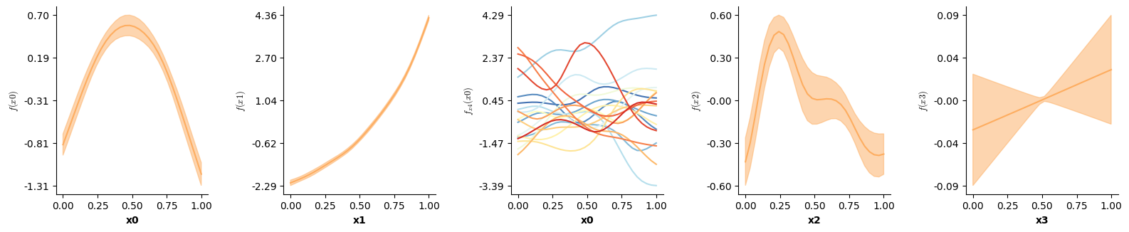
# For comparison: the GAMMLSS estimates
fig = plt.figure(figsize=(5*single_size,single_size),layout='constrained')
axs = fig.subplots(1,5,gridspec_kw={"wspace":0.1})
plot(gaumlss_model2,axs=axs[:3])
plot(gaumlss_model2,axs=axs[3:],dist_par=1)
Important: while the L-qEFS update provides quantities that can be used to obtain confidence intervals (see the plot above), these are unlikely to have the same good coverage achieved by more theoretically complex algorithms (i.e., Newton’s method - also implemented by the GSMM class but requiring users to code up the gradient and Hessian). Nevertheless, they can still offer an indication of the uncertainty in different effects.
Proportional Hazard models
The GSMM class also supports estimation of multivariate additive models and proportional hazard models - both via the L-qEFS update and via Newton’s method (currently only for hazard models). Wood et al. (2016) have the details on these models. This section outlines how to estimate a proportional hazard model and how to visualize the estimated survival functions. We start with simulating some data:
# Simulate some data
sim_dat = sim3(500,2,c=1,seed=0,family=PropHaz([0],[0]),binom_offset = 0.1,correlate=False)
The PropHaz family implements the GSMMFamily class. In contrast to our previous simple example - this family requires two extra arguments:
a vector of unique event times
uta vector indexing the unique event time in
utobserved on the corresponding trial
Below, we create these two vectors:
# Prep everything for prophaz model

# Create index variable for residual ordering
sim_dat["index"] = np.arange(sim_dat.shape[0])

# Now re-order
sim_dat = sim_dat.sort_values(['y'],ascending=[False])
sim_dat = sim_dat.reset_index(drop=True)
print(sim_dat.head(),np.mean(sim_dat["delta"]))

u,inv = np.unique(sim_dat["y"],return_inverse=True)
ut = np.flip(u)
r = np.abs(inv - max(inv))
res_idx = np.argsort(sim_dat["index"].values)

# And create the family
PropHaz_fam = PropHaz(ut,r)
              y        x0        x1        x2        x3       eta  delta  \
0  29805.378136  0.499973  0.561587  0.056349  0.269721 -1.623298      1
1  29137.580996  0.732006  0.182843  0.052817  0.961029 -3.909978      1
2  29020.603591  0.266130  0.687415  0.800972  0.745394 -1.178566      1
3  28162.338874  0.777544  0.482538  0.996186  0.296208 -3.788008      1
4  27493.457712  0.105495  0.022611  0.457104  0.393151 -2.946211      1

   index
0    208
1    109
2    104
3    422
4     69   0.836
Now we can set up the formula of the survival model. Note, that a survival model only requires specifying a single formula - which also cannot include an intercept term:
# Now specify formula and model
sim_formula_m = Formula(lhs("delta"),
                        [f(["x0"]),f(["x1"]),f(["x2"]),f(["x3"])],
                        data=sim_dat)

model = GSMM([copy.deepcopy(sim_formula_m)],PropHaz_fam)
Now we can fit the model - by default the fit method of a GSMM attempts to rely on Newton’s method - so we dont have to specify anything else and can just call fit:
# Fit with Newton
model.fit(progress_bar=False)
When working with survival models, we are usually interested in visualizing the survival functions. Below we show how this can be achieved using the PropHaz family’s .get_survival method:
# Now get estimate of survival function and see how it changes with x0
new_dat = pd.DataFrame({"x0":np.linspace(0,1,5),
                        "x1":np.linspace(0,1,5),
                        "x2":np.linspace(0,1,5),
                        "x3":np.linspace(0,1,5)})

# Get model matrix using only f0
_,Xt,_ = model.predict(use_terms=[0],n_dat=new_dat)

# Now iterate over all time-points and obtain the predicted survival function + standard error estimate
# for all 5 values of x0:
S = np.zeros((len(ut),Xt.shape[0]))
VS = np.zeros((len(ut),Xt.shape[0]))
for idx,ti in enumerate(ut):

    # Su and VSu are of shape (5,1) here but will generally be of shape (Xt.shape[0],1)
    Su,VSu = PropHaz_fam.get_survival(model.coef,model.get_mmat(),sim_formula_m.y_flat[sim_formula_m.NOT_NA_flat],
                                    ti,Xt,model.lvi.T@model.lvi)
    S[idx,:] = Su.flatten()
    VS[idx,:] = VSu.flatten()

# Now we can plot the estimated survival functions + approximate cis:
for xi in range(Xt.shape[0]):

    plt.fill([*ut,*np.flip(ut)],
            [*(S[:,xi] + 1.96*VS[:,xi]),*np.flip(S[:,xi] - 1.96*VS[:,xi])],alpha=0.5)
    plt.plot(ut,S[:,xi],label=f"x0 = {new_dat["x0"][xi]}")
plt.legend()
plt.xlabel("Time")
plt.ylabel("Survival")
plt.show()
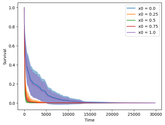
# Note how the main effect of x0 is reflected in the plot above:
plot(model,which=[0])
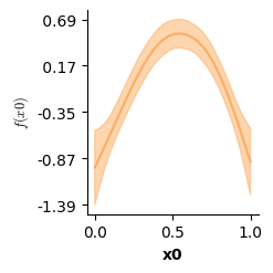
Residual plots can again be created via plot_val from mssmViz - by default Martingale residuals are returned (see Wood, 2017) for Proportional Hazard models. The example below also illustrates the use of the gsmm_kwargs and gsmm_kwargs_pred arguments of the plot_val function - see the doc string of the function for more details!
fig = plt.figure(figsize=(3*single_size,single_size),layout='constrained')
axs = fig.subplots(1,3,gridspec_kw={"wspace":0.2})

# Note the use of `gsmm_kwargs_pred={}` to ensure that the re-ordering is not applied to the plot against predicted values
plot_val(model,gsmm_kwargs={"reorder":res_idx},gsmm_kwargs_pred={},ar_lag=25,axs=axs)

# Can also get Deviance residuals:
fig = plt.figure(figsize=(3*single_size,single_size),layout='constrained')
axs = fig.subplots(1,3,gridspec_kw={"wspace":0.2})

plot_val(model,gsmm_kwargs={"reorder":res_idx,"resid_type":"Deviance"},gsmm_kwargs_pred={"resid_type":"Deviance"},ar_lag=25,axs=axs)
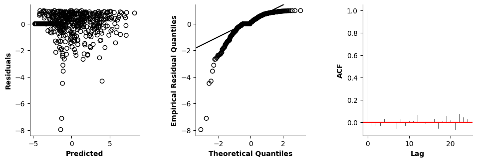
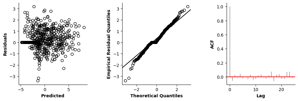
References
B-Splines and Difference Penalty bases:
Eilers, P., & Marx, B. (1996). Flexible smoothing with B-splines and penalties. Statistical Science, 11(2), 89–121. https://doi.org/10.1214/ss/1038425655
Eilers, P., & Marx, B. (2010). Splines, knots, and penalties. https://doi.org/10.1002/WICS.125
GAMM Estimation as implemented by mssm:
Wood, S. N. (2006). Low‐Rank Scale‐Invariant Tensor Product Smooths for Generalized Additive Mixed Models. Biometrics, 62(4), 1025–1036. https://doi.org/10.1111/j.1541-0420.2006.00574.x
Wood, S. N. (2011). Fast stable restricted maximum likelihood and marginal likelihood estimation of semiparametric generalized linear models: Estimation of Semiparametric Generalized Linear Models. Journal of the Royal Statistical Society: Series B (Statistical Methodology), 73(1), 3–36. https://doi.org/10.1111/j.1467-9868.2010.00749.x
Wood, S. N., Scheipl, F., & Faraway, J. J. (2013). Straightforward intermediate rank tensor product smoothing in mixed models. Statistics and Computing, 23(3), 341–360. https://doi.org/10.1007/s11222-012-9314-z
Wood, S. N., Goude, Y., & Shaw, S. (2015). Generalized additive models for large data sets. Journal of the Royal Statistical Society: Series C (Applied Statistics), 64(1), 139–155. https://doi.org/10.1111/rssc.12068
Wood, S. N., Pya, N., & Säfken, B. (2016). Smoothing Parameter and Model Selection for General Smooth Models. Journal of the American Statistical Association, 111(516), 1548–1563. https://doi.org/10.1080/01621459.2016.1180986
Wood, S. N. (2016). Just Another Gibbs Additive Modeler: Interfacing JAGS and mgcv. Journal of Statistical Software, 75(7). https://doi.org/10.18637/jss.v075.i07
Wood, S. N., Li, Z., Shaddick, G., & Augustin, N. H. (2017). Generalized Additive Models for Gigadata: Modeling the U.K. Black Smoke Network Daily Data. Journal of the American Statistical Association, 112(519), 1199–1210. https://doi.org/10.1080/01621459.2016.1195744
Wood, S. N., & Fasiolo, M. (2017). A generalized Fellner-Schall method for smoothing parameter optimization with application to Tweedie location, scale and shape models. Biometrics, 73(4), 1071–1081. https://doi.org/10.1111/biom.12666
Krause et al. (submitted). The Mixed-Sparse-Smooth-Model Toolbox (MSSM): Efficient Estimation and Selection of Large Multi-Level Statistical Models. https://doi.org/10.48550/arXiv.2506.13132
GAMMLSS Estimation as implemented by mssm & Smoothing penalty uncertainty:
Rigby, R. A., & Stasinopoulos, D. M. (2005). Generalized Additive Models for Location, Scale and Shape. Journal of the Royal Statistical Society Series C: Applied Statistics, 54(3), 507–554. https://doi.org/10.1111/j.1467-9876.2005.00510.x
Wood, S. N., Pya, N., & Säfken, B. (2016). Smoothing Parameter and Model Selection for General Smooth Models. Journal of the American Statistical Association, 111(516), 1548–1563. https://doi.org/10.1080/01621459.2016.1180986
Krause et al. (submitted). The Mixed-Sparse-Smooth-Model Toolbox (MSSM): Efficient Estimation and Selection of Large Multi-Level Statistical Models. https://doi.org/10.48550/arXiv.2506.13132
Kernel penalties & Penalty-based model selection:
Marra, G., & Wood, S. N. (2011). Practical variable selection for generalized additive models. Computational Statistics & Data Analysis, 55(7), 2372–2387. https://doi.org/10.1016/j.csda.2011.02.004
Whole-interval CIs:
Simpson, G. (2016). Simultaneous intervals for smooths revisited. Accessed at: https://fromthebottomoftheheap.net/2016/12/15/simultaneous-interval-revisited/
GAMMS in general & Overview:
Wood, S. N. (2020). Inference and computation with generalized additive models and their extensions. TEST, 29(2), 307–339. https://doi.org/10.1007/s11749-020-00711-5
Wood, S. N. (2017). Generalized Additive Models: An Introduction with R, Second Edition (2nd ed.). Chapman and Hall/CRC.